Mesoscale wind stress-SST coupling induced feedback to the ocean in the western coast of South America*

Chaoran CUI , Rong-Hua ZHANG ,3,4 , , Yanzhou WEI, Hongna WANG

1 Key Laboratory of Ocean Circulation and Waves, Institute of Oceanology, and Center for Ocean Mega-Science, Chinese Academy of Sciences, Qingdao 266071, China

2 University of Chinese Academy of Sciences, Beijing 100049, China

3 Qingdao National Laboratory for Marine Science and Technology, Qingdao 266000, China

4 Center for Excellence in Quaternary Science and Global Change, Chinese Academy of Sciences, Xi’an 710061, China

5 State Key Laboratory of Satellite Ocean Environment Dynamics, Second Institute of Oceanography, Ministry of Natural Resources, Hangzhou 310012, China

Abstract The feedback induced by mesoscale wind stress-SST coupling to the ocean in the western coast of South America was studied using the Regional Ocean Modeling System (ROMS). To represent the feedback, an empirical mesoscale wind stress perturbation model was constructed from satellite observations,and was incorporated into the ocean model. Comparing two experiments with and without the mesoscale wind stress-SST coupling, it was found that SST in the mesoscale coupling experiment was reduced in the western coast of South America, with the maximum values of 0.5 ℃ in the Peru Sea and 0.7 ℃ in the Chile Sea. A mixed layer heat budget analysis indicates that horizontal advection is the main term that explains the reduction in SST. Specifically, the feedback induced by mesoscale wind stress-SST coupling to the ocean can enhance vertical velocity in the nearshore area through the Ekman pumping, which brings subsurface cold water to the sea surface. These results indicate that the feedback due to the mesoscale wind stress-SST coupling to the ocean has the potential for reducing the warm SST bias often seen in the large-scale climate model simulations in this region.

Keyword: mesoscale air-sea coupling; western coast of South America; ocean model simulations; cooling eff ect; warm bias

1 INTRODUCTION

Mesoscale air-sea coupling is a salient process that is prominent in the regions with energetic eddies and fronts. It is often characterized by a positive correlation between sea surface temperature (SST) perturbations(SSTmeso) and wind stress perturbations (WSmeso) at a typical length of 10–100 km. The influence of mesoscale SST perturbations on the surface wind stress was previously observed by Sweet et al. (1981),who found that the magnitude of cross-front wind stress increased when the wind passed from cold to warm water in the Gulf Stream. Mesoscale air-sea coupling is also characterized by a linear correlation between wind stress divergence (curl) perturbations Div(WS)meso(Curl(WS)meso) and downwind(crosswind) SST gradient perturbations ∇downSSTmeso( ∇crossSSTmeso) (Chelton et al., 2004, 2007). These relationships have been verified by observations and model simulations (Shaw et al., 1999; Chelton et al.,2001; Bourras, 2004; O’Neill et al., 2005; Small et al.,2008; Castelao, 2012; O’Neill, 2012).

The mesoscale air-sea coupling can be well described by two mechanisms (Chelton et al., 2007;Small et al., 2008; Chelton and Xie, 2010; Desbiolles et al., 2018; Gao et al., 2019). The first is related to downwind momentum transport. SSTmesocan modify the turbulent mixing within the marine atmospheric boundary layer, and then the downward momentum transport is changed and generates advective acceleration of near-surface wind from cool to warm SST and deceleration of near-surface wind from warm to cool SST. The second mechanism is related to the sea level pressure adjustment. Observations show that WSmesoin the upstream (downstream) of warm SSTmesois accelerated (decelerated) due to sea level pressure anomalies above SSTmeso.

A strong eastern boundary upwelling exists in the western coast of South America (Albert et al., 2010;Oerder et al., 2015). The strong wind-forced upwelling supplies rich nutrients in this region, producing a productive ecosystem that provides much of the world’s fish catch (Chavez et al., 2008). Furthermore,this region plays an important role in the global climate because ofits eff ect on the El Niño-Southern Oscillation (Ma et al., 1996). Model simulations have been a powerful approach to understand and predict the upwelling system in this region and its climate eff ects. However, there is a consistent warm SST bias in most of climate model simulations in this region(Zuidema et al., 2016; Zhu and Zhang, 2018, 2019;Zhang et al., 2020). This bias in the tropical ocean may be aff ected by cloud liquid water path and stratus cloud coverage represented in atmospheric models,which leads to an excessive amount of solar radiation that is received at the sea surface (Ma et al, 1996;Davey et al., 2002; Meehl et al., 2005; Huang et al.,2007; Hu et al., 2011).

Note that strong mesoscale air-sea coupling occurs in the western coast of South America because of intense mesoscale eddy activities. Previous studies have showed that mesoscale wind stress-SST coupling can have important feedback to the atmosphere and ocean (Zhang and Busalacchi, 2008; Hogg et al.,2009; Frenger et al., 2013; Zhang et al., 2014; Zhang,2014; Ma et al., 2016; Wei et al., 2017). Piazza et al.(2016) showed the mesoscale coupling had an upscale eff ect on the tropospheric wind and storm in the Gulf Stream. Particularly, as the change in wind stress curl induced by mesoscale coupling can impact the Ekman pumping, the mesoscale wind stress-SST coupling can exert an important feedback to the upwelling system, which may aff ect SST in this region (Bakun,1990; Jin et al., 2009; Albert et al., 2010; Gaube et al.,2015; Seo et al., 2016). Indeed, Penven et al. (2005)showed that the warm SST bias in climate models might be a consequence of their incapacity to accurately resolve the nearshore upwelling and eddy activities. Therefore, it is necessary to study the feedback induced by the mesoscale air-sea coupling to the ocean in this region, which may potentially reduce the warm SST bias in many climate models.

Using a high resolution Weather Research and Forecasting (WRF) and Nucleus for European Modeling of the Ocean (NEMO) model, Oerder et al.(2016) showed that WSmesoresponse to SSTmesoin the western coast of South America was mainly attributed to turbulent momentum transport in the atmospheric boundary layer, with the coupling coeffi cient between WSmesoand SSTmesoin austral winter being larger than that in austral summer. They also showed that the intensity of mesoscale eddy activities was reduced if the eff ect of surface ocean current on the wind stress was taken into account in the model (Oerder et al.,2018). However, there are few studies focusing on the feedback induced by the mesoscale wind stress-SST coupling in this region. Therefore, we aim to study the feedback induced by mesoscale wind stress-SST coupling to the ocean in the western coast of South America. As ocean-only models and coarse-resolution climate models cannot adequately represent the characteristics of mesoscale wind stress-SST coupling(Bryan et al., 2010), we explore an empirical approach to parameterize WSmesofrom SSTmesogradients, and incorporate it in the ocean model to examine the eff ect on ocean simulation.

The paper is organized as follows: Section 2 describes the empirical wind stress perturbation model, the ocean model and experimental configuration. Section 3 reports the feedback induced by the mesoscale wind stress-SST coupling to the ocean simulation in the western coast of South America. Section 4 examines the processes by which the mesoscale coupling impacts the SST, and Section 5 presents a summary.

2 METHODOLOGY

2.1 Observed data

The satellite data are used to quantify the mesoscale SST-wind stress coupling relationship in this study.The daily wind stress data are derived from Quick Scatterometer (Quik-SCAT, Version 4) which are launched from July 1999 to November 2009. The AMSR-E SST data are available from June 2002 to September 2011. For this study, we use the daily data with spatial resolution of 0.25° for period from June 2002 to November 2009. All of the data are obtained from the Asia-Pacific Data-Research Center (APDRC)of the University of Hawaii.

2.2 An empirical wind stress perturbation model

in whichm=d/dmax,dis the distance between target point and a surrounding point,dmaxis the maximum distance between target point and each point in the spatial filter window.

The magnitude of the derived perturbations depends on the half-span parameter used in the LOESS method. In order to extract the mesoscale perturbations effi ciently in the western coast of South America, the half-span parameter is taken as 10°according to previous results (Cui et al., 2020).

To determine WSmesoeff ectively for use in the ocean model, the Tikhonov regularization method is used to calculate WSmesofrom the Curl(WSmeso) and Div(WSmeso), which are approximated from modeled∇downSSTmesoand ∇crossSSTmesousing their empirical relationships obtained from satellite observations.Details of the method can be found in Wei et al. (2017,2018) and Cui et al. (2020).

2.3 Ocean model

The ocean model used in this study is the Regional Ocean Modeling System (ROMS) version 3.4. ROMS is a three-dimensional, free surface and terrainfollowing numerical model. It solves hydrostatic and primitive equations using a short time step for the surface elevation and barotropic momentum equations, and a longer time step for 3D temperature,salinity and baroclinic momentum equations (Song and Haidvogel, 1994; Shchepetkin and McWilliams,2005). ROMS provides several schemes for mixing parameterizations. This study takes the harmonic mixing scheme for horizontal mixing and the Mellor/Yamada Level-2.5 closure parameterization scheme for vertical mixing (Wajsowicz, 1993). Horizontal tracer and momentum advection are treated using a third-order upstream discretization scheme. The vertical advection is evaluated using the fourth-order centered discretization scheme. Details of the ROMS computational algorithms are described by Shchepetkin and McWilliams (2005).

To resolve the mesoscale phenomenon in the region and its interactions with basin-scale ocean circulation in the tropical Pacific, we configured a nested modeling system using ROMS with two diff erent domains at high and low spatial resolutions,respectively. The larger domain covers the whole tropical Pacific from 35°S to 35°N and from 100°E to 70°W with a horizontal grid resolution of 1/2°×1/2°cosΦ(Φis latitude). The small inner domain extends from 30°S to 0°N and from 95°W to 70°W in the western coast of South America; the horizontal grid resolution ofinner domain is 1/8°×1/8°cosΦ(Φis latitude). In the vertical direction, there are 40 levels(s-coordinate) of the inner domain with higher vertical resolution near the surface and bottom (Song and Haidvogel, 1994; Haidvogel et al., 2008). The bottom topographies in both domains are obtained from the Global 2-min Gridded Topographic Data ETOPO2.The ETOPO2 data set was generated from a digital database of seafloor and land elevations, which includes the satellite altimeter data, shipboard echosounding measurements, and data from global digital elevation model. Note that the eastern boundary is closed and other three (northern, southern, and western) boundaries are open for both the domains.The depth ranges from 75 m to 5 000 m. To make long-term integrations more stable, radiation-nudging boundary conditions are used with a 360-day time scale for outflow and 3-day time scale for inflow. The time steps are 30 s for the 2-D barotropic equations,and 300 s for the 3-D baroclinic equations.

The Quik-SCAT monthly mean surface wind fields during 2003–2008 are used to force the ocean model.Air-sea fluxes are calculated by the bulk formulae from atmosphere parameters (the National Center for Environmental Prediction (NCEP) reanalysis product during 1985–2015, including monthly mean relative humidity, solar shortwave radiation, longwave radiation, precipitation, surface air pressure, and surface air temperature). The initial and boundary conditions for the larger-domain model are specified from the World Ocean Atlas 2009 (WOA2009), which is a set of objectively analyzed climatological hydrographic data for ocean parameters from 0 m at the surface to 5 500 m at the bottom. The largerdomain model is run for 30 years and its monthly mean outputs provide initial and boundary conditions for the inner-domain model. The inner-domain model is also run for 30 years to get a quasi-equilibrium state of 3-D velocity, temperature, and salinity, as well as the 2-D sea surface elevation.

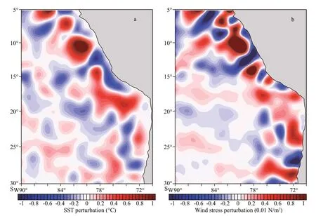
Fig.1 Spatially high pass filtered AMSR-E SST (a) and Quik-SCAT wind stress (b) magnitude in April 2007

2.4 Sensitivity experiment

To assess the feedback due to mesoscale coupling to the ocean in the western coast of South America,four experiments are designed. The first experiment is a control one with model settings described above.The second one is the mesoscale coupling experiment,in which the eff ect of mesoscale coupling is included by calculating the WSmesofrom its empirical model in ROMS. The WSmesois derived from Curl(WSmeso) and Div(WSmeso) which are approximated from modeled∇downSSTmesoand ∇crossSSTmesoat each time step. Then,the mesoscale wind speed perturbation (WSPDmeso) is obtained from the WSmesoand added to the monthly mean wind speed, which modifies the surface wind stress and heat flux based on the bulk formula.

Other two experiments are designed to investigate the separate feedback of mesoscale coupling to the ocean associated with heat flux and momentum flux,respectively. They are referred to as the HF-feedback experiment (only the influence of WSPDmesoon surface heat flux (HF) is considered) and the MFfeedback experiment (only the influence of WSmesoon surface wind stress (momentum flux; MF) is considered), respectively.These four experiments all start from the beginning of the 31styear of model simulation, and are run for 10 years to investigate the eff ect of mesoscale air-sea coupling on long-term mean ocean simulations.

3 FEEDBACK DUE TO MESOSCALE COUPLING TO THE OCEAN

3.1 Simulated mesoscale SST and wind stress perturbations

Figure 1 shows mesoscale perturbation fields of AMSR-E SST and Quik-SCAT wind stress magnitude in April 2007. The field of WSmesomagnitude is highly consistent with that of SSTmeso, and the wind slows down over cooler waters and speeds up over warmer waters. It is evident that the LOESS method can isolate the mesoscale signals effi ciently from the large-scale background field. Figure 2a–b shows the simulated long-term mean SSTmesoand WSmesoin the western coast of South America, respectively. It is clearly seen that the characteristic SSTmesoand WSmesofeatures in observations can be well captured. The regions with large SSTmesoare in the nearshore area of Peru Sea and Chile Sea both in the observations and simulated outputs. The reconstructed WSmesois closely related to that of simulated SSTmeso(Fig.2a–b). As shown in Fig.3, the coupling coeffi cient between SSTmesoand WSmesoin simulation (0.007 6 ℃/(N/m2)) is nearly equal to that in observations (0.006 5 ℃/(N/m2)).These results indicate that WSmesocan be well represented from the SSTmesousing the empirical model calculated by the Tikhonov’s regularization method.

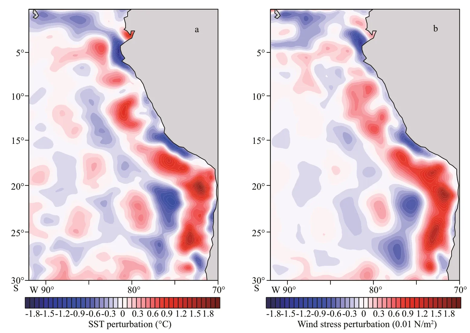
Fig.2 The simulatedmesoscale SST (a) and wind stress (b) magnitude perturbations which are averaged from the 31st to the 40th yearin ROMS

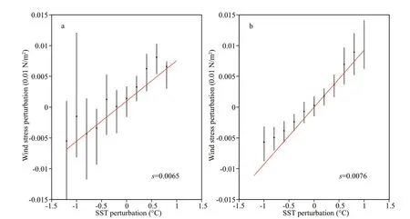
Fig.3 The coupling coeffi cients between wind stress and SST perturbations in observations (Quik-SCAT wind stress and AMSR-E SST data during 2003–2008) (a) and ROMS model simulation (b)

3.2 Feedback to SST

To diagnose the feedback induced by mesoscale coupling on SST, the mesoscale coupling experiment(described in Section 2.4) is conducted. Figure 4 shows the mean SST diff erence between the two experiments. Obviously, SST is reduced in the off shore areas of the Peru and Chile Sea in the mesoscale coupling experiment. The reduced maximum values of SST can reach 0.5 ℃ in the Peru Sea and 0.7 ℃ in the Chile Sea. It is worth noting that there is positive SST diff erence in nearshore sea area.

The physical processes that lead to the SST diff erence are examined by the mixed layer (ML) heat budget analysis. The mixed layer depth (MLD) is defined as the depth at which the density increases by 0.125 kg/m3from the sea surface (Chelton et al.,2007). The vertically averaged ML heat budget equation is derived from the conservation of temperature equation:

wherehis MLD;Tandvare temperature and horizontal currents; subscriptarepresents quantities that are vertically averaged between the surface andh;ρis the density of seawater;Cpis heat capacity of sea water;Qnetis the diff erence between downward surface heat flux and shortwave radiation transmitted through the bottom of MLQpen;weis entrainment velocity across the bottom of ML, calculated by:

in whichw-his the vertical velocity at the bottom of the mixed layer.Qpenis calculated by:

in whichQshortis the shortwave radiation, andQdiffis the diff usive heat flux at the bottom of ML:

in whichKzis the function of Richardson number.Details of the computation of heat budget in the ML were described by Huang et al. (2010).

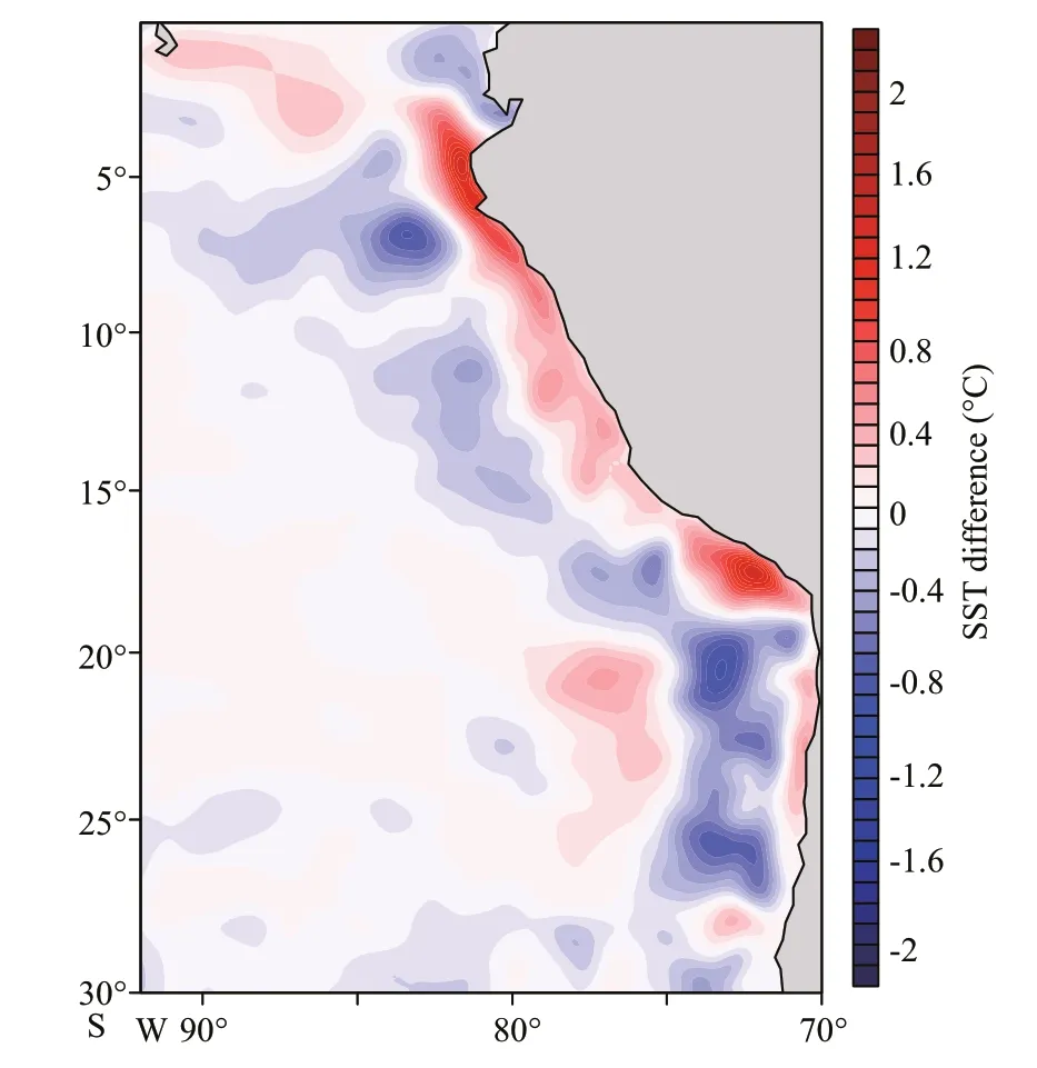
Fig.4 The mean SST diff erence between the mesoscale coupling experiment and control experiment

The left-hand side of Eq.3 is the ML temperature tendency, which is determined by terms on the righthand side. The first term on the right-hand side is the horizontal advection caused by depth-averaged current. The second term is the vertical entrainment.The third and fourth terms are the adjusted surface heat flux and vertical heat diff usion at the bottom of ML, respectively. Figure 5 shows the diff erences in each heat budget term between the mesoscale coupling experiment and control experiment. The diff erence in temperature tendency is not coherent and thus is not shown. The horizontal advection and surface heat flux are the main terms that explain the diff erence in SST(Fig.5a–b). The horizontal advection tends to decrease the SST in the off shore area and increase the SST in the nearshore area, which is consistent with SST diff erences induced by the feedback of mesoscale coupling. The surface heat flux has an opposite eff ect to the SST diff erence. The contributions of vertical entrainment and vertical heat diff usion terms are relatively small. They tend to damp the positive SST diff erence in the nearshore of Peru Sea (Fig.5c–d).

To further analyze the contribution of surface heat flux term to SST, the diff erences in latent heat flux,upward longwave radiation and sensible heat flux between the mesoscale coupling experiment and control experiment are presented in Fig.6. The latent heat flux is aff ected by wind speed and the temperature diff erence between the atmosphere and ocean surface based on the bulk flux formulae. As shown in Fig.6a,the diff erence in latent heat flux is closely related to that in SST (Fig.4), which means the eff ect due to the SST diff erence on latent heat flux is more important than wind speed in this region. The changed upward latent heat flux in turn acts to damp the SST diff erence.The similar results are found in upward longwave radiation and sensible heat flux (Fig.6b–c). It can be concluded that surface heat flux mainly acts to damp the SST diff erence in the western coast of South America; a similar case can be seen in the Kuroshio extension (Wei et al., 2017).

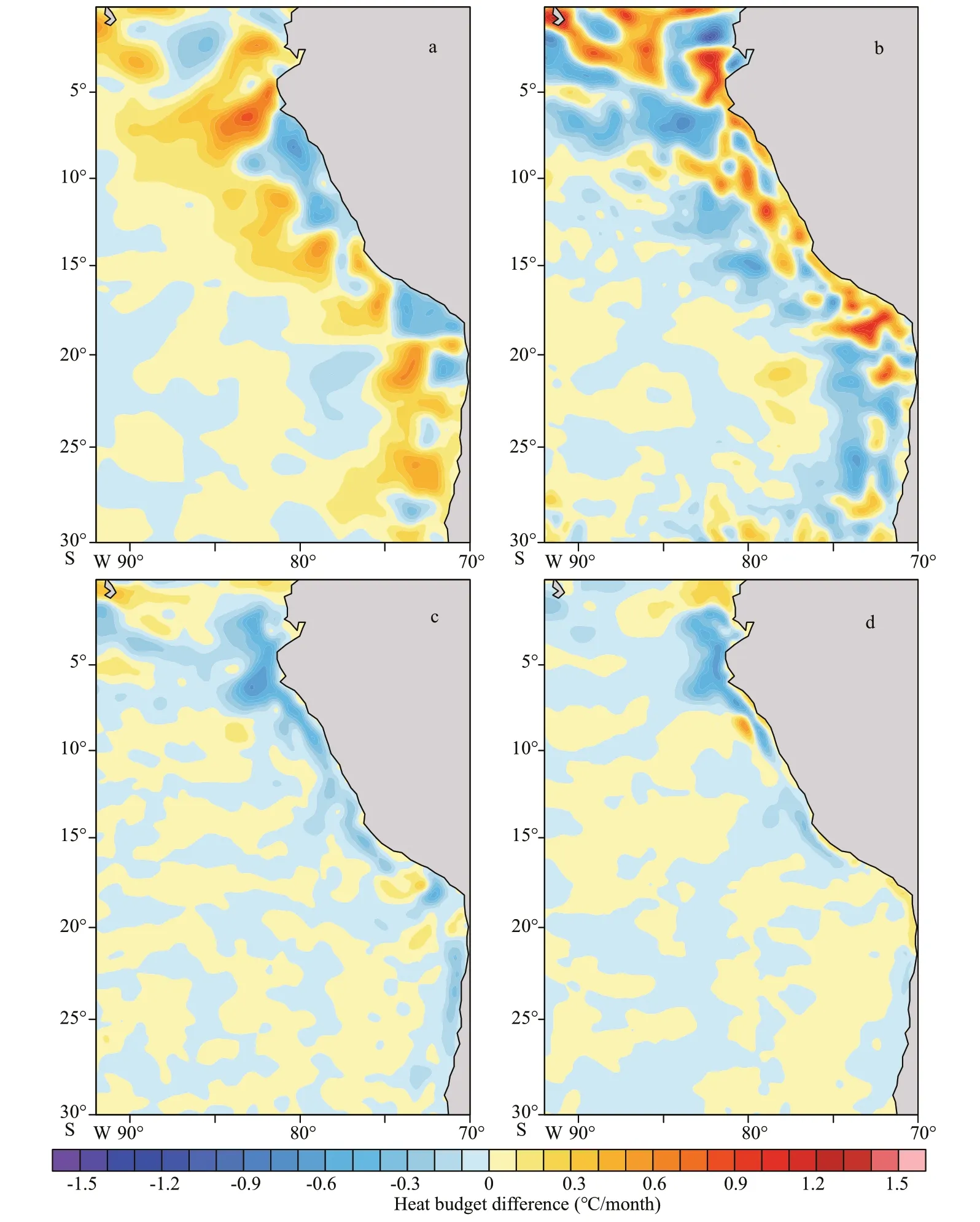
Fig.5 The diff erences in surface heat flux (a), horizontal advection (b), vertical entertainment (c), and vertical diff usion (d)in mixed layer heat budget equation between the mesoscale coupling experiment and control experiment

3.3 Feedback to ocean current

Figure 7 shows the long-term mean horizontal current in the control experiment and their diff erences between the mesoscale coupling experiment and control experiment. The results are vertically averaged in the mixed layer. Because of the strong westward wind, there is strong zonal off shore current in the western coast of South America (Fig.7a). The meridional current is northward in the nearshore area(Fig.7c). The mesoscale coupling exerts a profound feedback to horizontal current. Consistent with the negative WSmesoinduced by negative SSTmesoin the nearshore sea, the meridional and zonal current velocities are both weakened in these regions (Fig.7b& d). As the diff erence in SST is mainly determined by horizontal advection, the weakened horizontal currents in the nearshore sea is responsible for the positive SST diff erence.

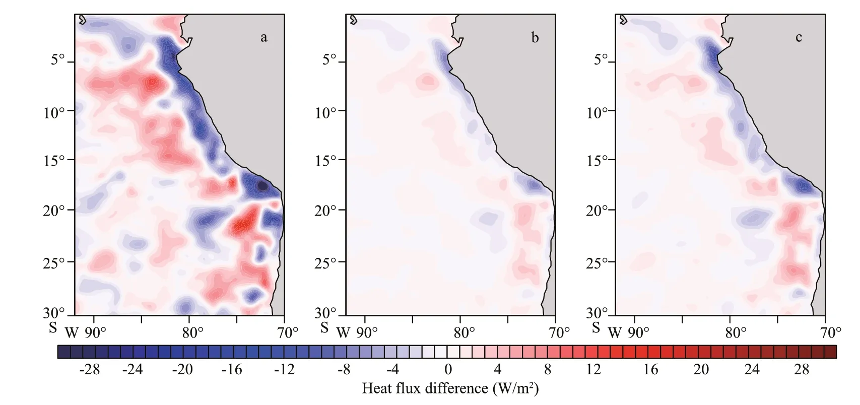
Fig.6 The diff erences in latent heat flux (a), upward longwave radiation (b), and sensible heat flux (c) between the mesoscale coupling experiment and control experiment

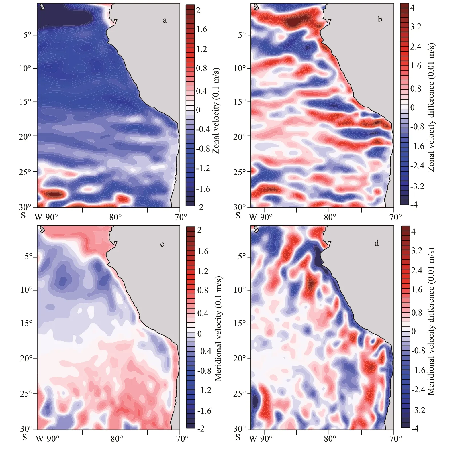
Fig.7 The long-term mean zonal (a) and meridional (c) current components in the control experiment; the diff erences in zonal (b) and meridional (d) current components between the mesoscale coupling experiment and control experiment

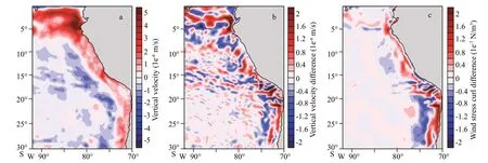
Fig.8 The long-term mean vertical current component in the control experiment (a); the diff erence in vertical current component between the mesoscale coupling experiment and control experiment (b); the diff erence in wind stress curl between the mesoscale coupling experiment and control experiment (c)

The long-term mean vertical current component in the control experiment and its diff erence between the mesoscale coupling experiment and control experiment are shown in Fig.8. The results are vertically averaged in the mixed layer. The vertical flow is upward in the nearshore sea area and downward in the off shore sea area (Fig.8a). When the feedback induced by mesoscale coupling to the ocean is incorporated into the model simulation, it is obvious that upward vertical velocity is strengthened in the nearshore sea (Fig.8b). Previous studies have found that Ekman pumping can be modulated by the curl of WSmesoespecially in the region with intense mesoscale eddy activities (Gaube et al., 2015; Seo et al., 2016;Seo, 2017). To examine whether the diff erence in vertical velocity is related to the Ekman pumping induced by curl of WSmeso, the diff erence in wind stress curl between the mesoscale coupling experiment and control experiment is given in Fig.8c. It shows that the diff erence in vertical current is consistent with that in wind stress curl, indicating the diff erence in vertical velocity is mainly attributed to the diff erence in Ekman pumping induced by curl of WSmeso. In summary, the ocean current velocity is substantially aff ected by mesoscale coupling in the western coast of South America. The strengthened Ekman pumping can bring subsurface cold water to the sea surface and lead to the cooling of SST.

3.4 The seasonality of the feedback eff ect

The feedback eff ect of mesoscale wind stress-SST coupling on the ocean displays seasonal variation.Figure 9 shows the diff erences in SST between the mesoscale coupling experiment and control experiment in four seasons. The diff erence in SST is relatively large in austral summer (February–April) and small in austral winter (August–October). By analyzing heat budget terms in the ML, it is found that the cooling tendency in SST is attributed to horizontal advection,vertical entrainment, and vertical heat diff usion both in austral summer and winter. The contributions of horizontal advection, vertical entrainment, and vertical heat diff usion terms in austral summer are larger than those in winter. The vertical velocity diff erences induced by feedback of the mesoscale coupling in four seasons are given in Fig.10. As discussed above, the diff erence in vertical velocity is mainly attributed to Ekman pumping induced by curl of WSmeso. Thus, the diff erence in vertical velocity is consistent with that in WSmesocurl in all seasons (not shown). Figure 10 also shows the upwelling in the off shore area of Peru Sea in austral winter is weaker than that in summer. The weakened upwelling reduces the transport of subsurface cold water to sea surface, which can be one factor inducing the less cooled SST in austral winter.

4 SENSITIVITY EXPERIMENT

We have shown that the incorporation of mesoscale coupling into the model can lead to SST diff erence in the western coast of South America. The diff erence in SST can be determined by momentum flux (MF) and heat flux (HF), since mesoscale wind forcing can alter the surface wind stress and surface heat flux directly.To examine the way by which the mesoscale coupling impacts the SST, the HF-feedback experiment (only the influence of WS meso on surface heat flux is considered) and MF-feedback experiment (only the influence of WSmesoon surface wind stress is considered) are conducted (Table. 1), and results are presented in this section. Details of two experiments are described in Section 2.4.

Figure 11 shows the diff erences in SST between the two sensitivity experiments and control experiment. In the MF-feedback experiment, the reduced maximum values of SST are about 0.5 ℃both in Peru Sea and Chile Sea (Fig.11a). In the HFfeedback experiment, the regions with large diff erence in SST are mainly in the Chile Sea with maximum reduced value being about 0.3 ℃ (Fig.11b). The SST diff erence between the mesoscale coupling experiment and control experiment is generally a sum of the SST diff erences between the two sensitivity experiments and control experiment. Heat budget analysis also indicates that the SST diff erence is mainly determined by horizontal advection and surface heat flux in both the sensitivity experiments.

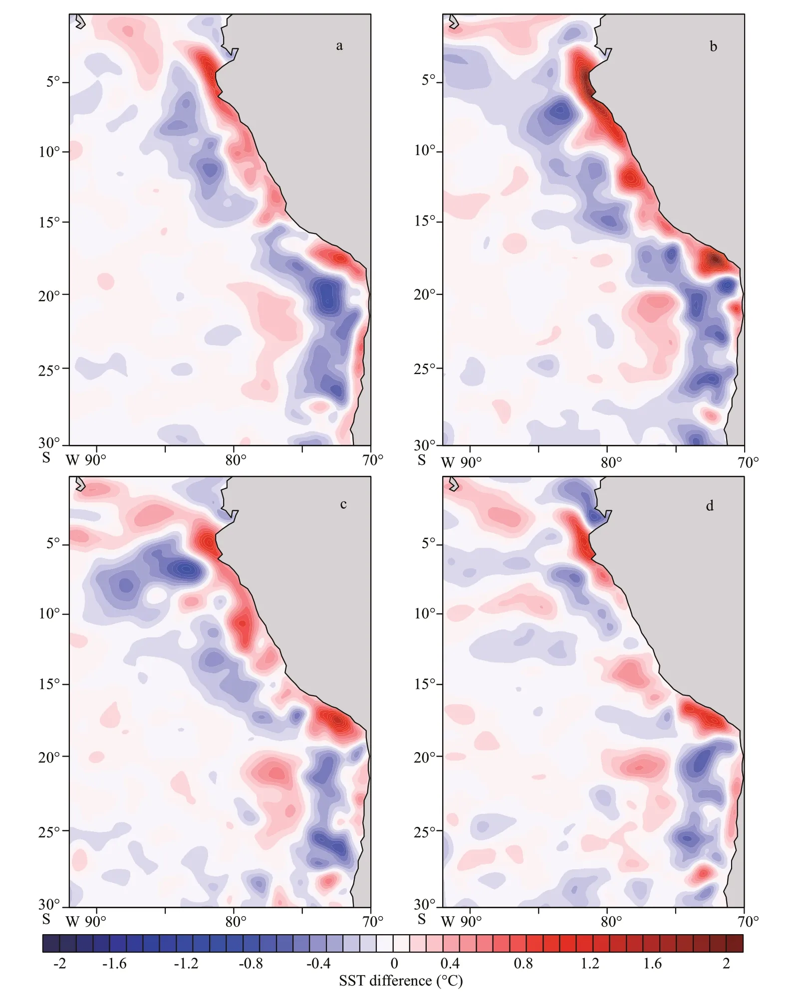
Fig.9 The diff erences in SST in austral spring (November–January) (a), austral summer (February–April) (b), austral autumn (May–July) (c), and austral winter (August–October) (d) between the mesoscale coupling experiment and control experiment

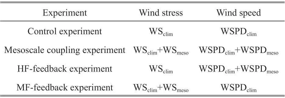
Table 1 The wind forcing specifications in the four experiments

In addition, the diff erences in sea surface heat flux between the two sensitivity experiments and control experiment are shown in Fig.12. The latent heat flux is aff ected by wind speed and temperature diff erence between the atmosphere and ocean surface. As wind speed is not allowed to be aff ected by wind speed perturbations due to SSTmesoin MF-feedback experiment, the diff erence in latent heat flux is well related to that in mean SST (Figs.11a & 12a). The similar results are found in the upward longwave radiation and sensible heat flux (Fig.12b & c). In HFfeedback experiment, the diff erence in latent heat flux(Fig.12d) is mainly determined by wind speed perturbations induced by SSTmeso, whereas the diff erences in upward longwave radiation and sensible heat flux are mainly determined by mean SST diff erence (Fig.12e & f).

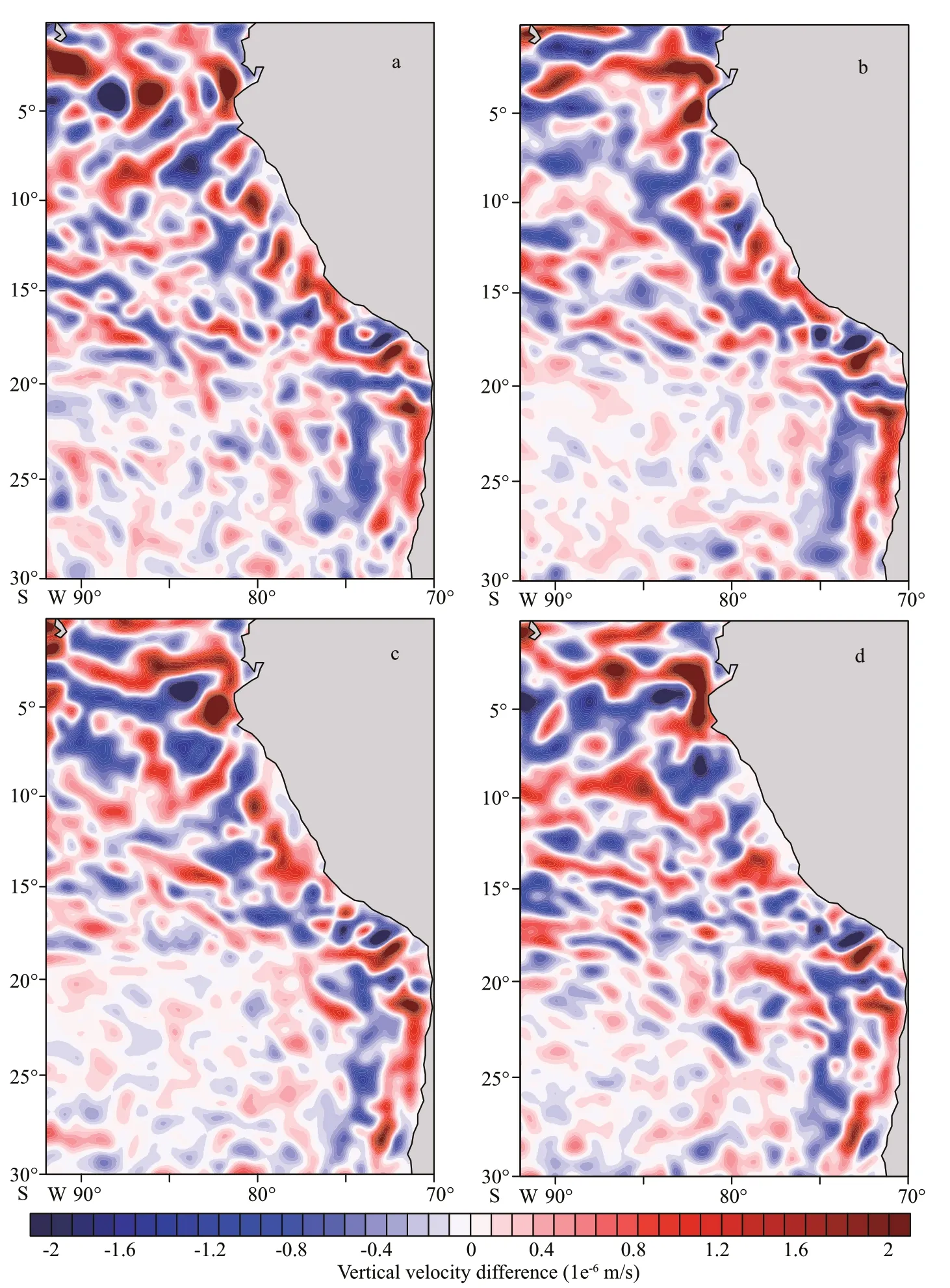
Fig.10 The diff erences in vertical current in austral spring (November–January) (a), austral summer (February–April) (b),austral autumn (May–July) (c), and austral winter (August–October) (d) between the mesoscale coupling experiment and control experiment

5 CONCLUSION AND DISCUSSION

In this work, the feedback eff ect induced by the mesoscale wind stress-SST coupling on the ocean in the western coast of South America is investigated by numerical simulations. Firstly, according to the coupling relationships between Div(WSmeso)(Curl(WSmeso)) and ∇downSSTmeso( ∇crossSSTmeso) derived from the satellite data, Div(WSmeso) and Curl(WSmeso)are obtained from SST gradient perturbations simulated from the ROMS. Then, WSmesois derived from Div(WSmeso) and Curl(WSmeso) by the Tikhonov regularization method and incorporated into the ROMS to represent its eff ect on the ocean. After including the feedback of mesoscale wind stress-SST coupling in the ROMS, SST can be reduced in the off shore area of the Peru and Chile Sea. The maximum reduced values can reach 0.5 ℃ in the Peru Sea and 0.7 ℃ in the Chile Sea.

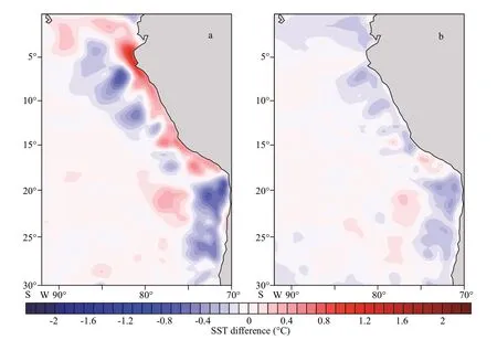
Fig.11 The diff erences in SST between the MF-feedback experiment and control experiment (a) and HF-feedback experiment and control experiment (b)

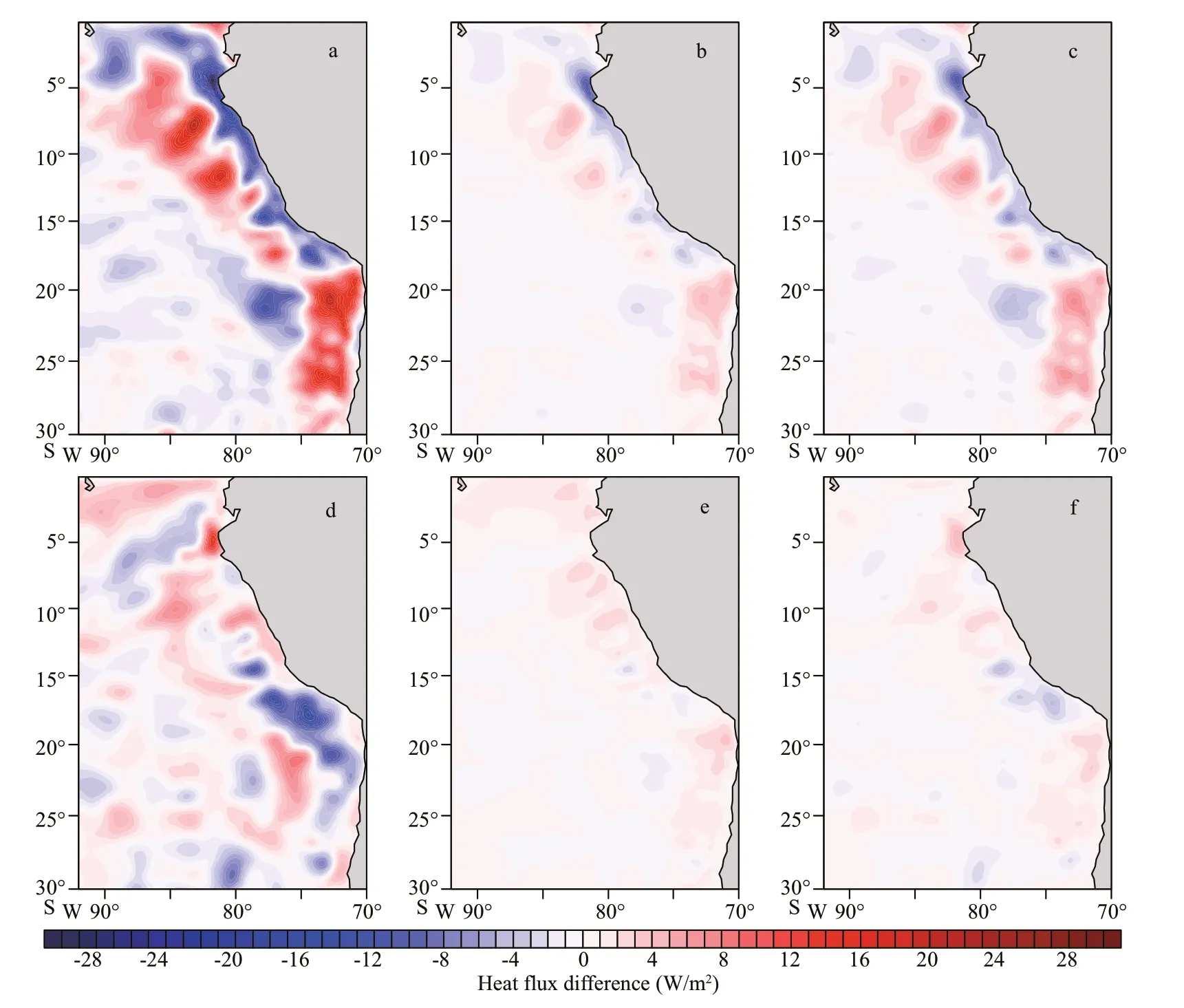
Fig.12 The diff erences in latent heat flux (a), upward longwave radiation (b), and sensible heat flux (c) between the MFfeedback experiment and control experiment; the diff erence in latent heat flux (d), upward longwave radiation (e),and sensible heat flux (f) between the HF-feedback experiment and control experiment

Based on the mixed layer heat budget analysis, we find that horizontal advection and surface heat flux are the main terms that explain the diff erence in SST between the mesoscale coupling experiment and control experiment. The horizontal advection term has a positive contribution to the SST diff erence with the cooling in off shore area and slightly warming in the nearshore area. However, the surface heat flux has a negative eff ect on the SST diff erence. Vertical entrainment and vertical heat diff usion act to damp the SST warming in the nearshore of Peru Sea. The feedback due to mesoscale coupling to the ocean also leads to strengthened vertical velocity in the nearshore sea area, which is mainly attributed to the Ekman pumping induced by curl of WSmeso.

The cooling SST induced by mesoscale wind stress-SST coupling is relatively large in austral summer (February–April) and small in austral winter(August–October). By analyzing the heat budget terms in the ML, it is found that the SST cooling is primarily contributed by the horizontal advection term both in austral summer and winter. Meanwhile,there is weaker upwelling in the off shore area of Peru Sea in austral winter than in austral summer. The weakened upwelling reduces the transport of subsurface cold water to sea surface; this can be one reason why SST is less cooled in austral winter.

The way by which the mesoscale coupling aff ects the SST in the western coast of South America is examined further by two sensitivity experiments. In the MF-feedback experiment (only the influence of WSmesoon surface wind stress is considered), the reduced values of SST are about 0.5 ℃ both in the Peru Sea and Chile Sea. In the HF-feedback experiment (only the influence of WSmesoon surface heat flux is considered), the regions with large SST diff erence (＞0.3 ℃) are mainly in the Chile Sea. By analyzing the heat budget terms in ML, horizontal advection and surface heat flux are also the main terms that explain the SST diff erences between the two sensitivity experiments and control experiment.

Thus, the mesoscale wind stress-SST coupling can have important feedback eff ect on the ocean in the western coast of South America. The feedback induced by mesoscale wind stress-SST coupling can reduce SST by a maximum of 0.5 ℃ in the Peru Sea and 0.7 ℃ in the Chile Sea, which may potentially reduce the warm SST bias in current climate models and improve the ocean simulations in the western coast of South America.

Although the computational application in this study is located in the western coast of South America,the empirical model constructed by the Tikhonov’s regularization method can be applicable to any regions and useful for the study of mesoscale coupling.As it is diffi cult to well simulate the atmospheric wind response to SSTmesoin the climate models with simulated coupling coeffi cient between WSmesoand SSTmesobeing smaller than observations (Bryan et al.,2010), the empirical model can be used to represent WSmesoin response to SSTmeso. This method can help shed light on better understanding of the physical processes that are involved in the mesoscale SSTwind coupling and improve the model simulations.

6 DATA AVAILABILITY STATEMENT

All the satellite data are obtained from the Asia-Pacific Data-Research Center (APDRC) of the University of Hawaii, which is available at http://apdrc.soest.hawaii.edu/las/v6/dataset?catitem=1. The model data and computer codes used in this paper are available from the authors (e-mail: rzhang@qdio.ac.cn).

7 ACKNOWLEDGMENT

The authors wish to thank the anonymous reviewers for their comments that helped to improve the original manuscript.