A physics-constrained deep residual network for solving the sine-Gordon equation

Jun Li(李军) and Yong Chen(陈勇)

1 Shanghai Key Laboratory of Trustworthy Computing,East China Normal University,Shanghai,200062,China

2 School of Mathematical Sciences,Shanghai Key Laboratory of PMMP,Shanghai Key Laboratory of Trustworthy Computing,East China Normal University,Shanghai,200062,China

3 College of Mathematics and Systems Science,Shandong University of Science and Technology,Qingdao,266590,China

4 Department of Physics,Zhejiang Normal University,Jinhua,321004,China

Abstract Despite some empirical successes for solving nonlinear evolution equations using deep learning,there are several unresolved issues.First,it could not uncover the dynamical behaviors of some equations where highly nonlinear source terms are included very well.Second,the gradient exploding and vanishing problems often occur for the traditional feedforward neural networks.In this paper,we propose a new architecture that combines the deep residual neural network with some underlying physical laws.Using the sine-Gordon equation as an example,we show that the numerical result is in good agreement with the exact soliton solution.In addition,a lot of numerical experiments show that the model is robust under small perturbations to a certain extent.

Keywords:sine-Gordon equation,deep residual network,soliton,integrable system

1.Introduction

Solving nonlinear evolution equations computationally plays a very important role in physics and engineering.Approximating these equations using deep learning rather than traditional numerical methods has been studied[1–3].Han et al[1]introduce a deep learning approach to approximate the gradient of the unknown solution.However,Raissi et al[2,3]approximate the latent solution using deep neural networks directly.Recently,we also explore the applications in other evolution equations such as the Burgers equation(it should be emphasized that strictly speaking,we just study kink-type solitary wave solutions to this equation),the Korteweg–de Vries(KdV)equation,the modified KdV equation,and the Sharma–Tasso–Olver equation[4,5]where these integrable equations have exact and explicit solutions to test the accuracy of the solutions via neural network methods.These data-driven solutions are closed analytic,differentiable and easy to be used in subsequent calculations compared with traditional numerical approaches.Moreover,compared with other traditional numerical approaches,the deep learning method does not require the discretization of spatial and temporal domains.

Some experiments show that the model in[2]could not approximate the solutions to some equations including highly nonlinear source terms such as sin(u)very well and then the model in[3]usually cannot represent the solution dynamics when using some activation functions.Thus,it is very interesting to improve the network framework to solve or alleviate these problems.In this paper,we propose a physics-constrained deep residual network that combines the deep residual neural network[6,7]with some underlying laws of physics.To our knowledge,it is the first framework combining the residual network with the underlying physical laws.This framework is easier to optimize than the classical feedforward networks.Moreover,it can increase gradient flow and then alleviate the gradient vanishing/exploding problems through adding the skip connection accordingly.It can also be used to train very deep networks to improve the performance of the network.By the way,here we just use a simple identity connection,more complex connections between these network layers are enable[8].

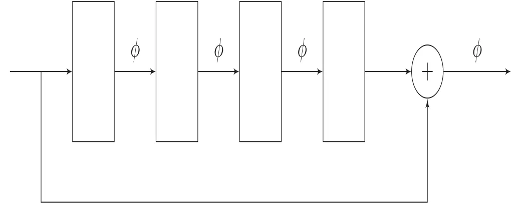
Figure 1.This figure sketches how the residual block works.

Specifically,in this paper,we just consider the sine-Gordon equation[9–11]which includes a highly nonlinear source term:

where the solution u is a function of the space variable x and the time variable t.Note that,through the coordinate transformationandwe can obtain another expression of this equation,namely,

The paper is organized as follows.In section 2,we propose the physics-constrained deep residual network and then present a new objective function.Then we give our main focus on the antikink solution to the sine-Gordon equation and the influence on the model of different settings such as noise,sampled data points,network layers and neurons in section 3.Finally,we conclude the paper in section 4.

2.Method

The residual block usually adds the output of a series of layers to the input of the block directly.Formally,in this work,we consider a residual block defined as

where W(n,i),b(n,i),i=1…4 are the weights and biases of the corresponding layers,respectively.Note that we use the activation function only in the hidden layers rather than the output layer.The identity map skips training from a few layers and connects to the output directly.If any layer hurt the performance of the network,then it will be skipped.So,this mechanism can be regarded as a kind of regularization.This results in training very deep neural networks without the problems caused by vanishing or exploding gradients.

In addition,we know that this residual structure is just a special case of the Euler forward scheme[12]

when h=1.See[13,14]for more detailed analyses from the viewpoints of dynamical systems and differential equations.

In this work,we approximate directly the unknown solution u using a deep residual network composed of three residual blocks and accordingly define a network

where these two networks share all parameters to be learned.The solution network is trained to satisfy the sine-Gordon equation(1)and corresponding initial/boundary conditions.With the help of the automatic differentiation techniques[15],equation(5)is embedded into a new loss function we propose here:

in order to utilize the underlying laws of physics to discover patterns fromexperimental/simulated data wheredenote the initial/boundary training data on the networku andspecify the collocation points for the networkf.The first term of the right hand side of equation(6)measures the difference between the true underlying and measured dynamics due to the noise that may be caused by different factors.Then the second term learns to satisfy f which prevents overfitting and denoises the data.In this paper,we just set λ=1 and choose the L-BFGS[16]algorithm to optimize the loss function(6).By the way,different from numerical differentiation,automatic differentiation possesses the advantages of small influence of noise and desirable stability,which will be observed in the next section.From equation(6),it can be observed that we use logcosh(x),which is also called smooth L1 function in some contexts,as the objective function.Through a simple calculus,we know that

Obviously,it is less affected by outliers and second-order differentiable everywhere.Moreover,the comparison of the difference between the absolute function,the square function and this function is given in figure 2.The logcosh function’s relation to the absolute function is just like the swish function’s relation to the rectified linear unit(ReLU).More discussions about the choice of the objective will be given in the next section.

Figure 2.The comparison of some common loss functions.

Some studies indicate that orthogonal initializations can restrict unit variance to improve the training procedure and the performance of architecture,but for most applications,Xavier initialization[17]used in this paper is enough.The activation function is what makes a neural network nonlinear.This nonlinearity property makes the network more expressive.Specifically,in this paper,the second-order derivatives of the solution with respect to the spatial variable x and the temporal variable t are needed,so ReLU(max{0,x})evidently does not work.Then,the data are usually rescaled to[−1,1].The sigmoid function(σ,1(1 +exp(−x))),however,restricts the output to[0,1].Thus,this function also does not work well.Moreover,most of the derivative values of this type of S-shaped functions including σ and tanh tend to 0 which will lose too much information and lead to the vanishing gradient problem to some extent.In addition,ReLU can not represent complicated and fine-grained details.Some numerical experiments demonstrate that they indeed cannot recover the solution dynamics correctly.We think that other different choices of weight initializations and data normalizations may also affect the selection of the activation functions.So,in this paper,we choose some periodic functions such as the sinusoid functions as the activation functions[18].For sin(x)which is zero centered,its derivativecos(x)is just a shifted sine function.

All experiments in this work are conducted on a Mac-Book Pro computer with 2.4 GHz Dual-Core Intel Core i5 processor.

3.Numerical Results

The soliton phenomena exist widely in physics,biology,communication and other scientific disciplines.The soliton solution(namely,kink or antikink)of the sine-Gordon equation we mention here,which is distinctly different from the KdV soliton(bell shaped),represents topologically invariant quantities in a system.Specifically,the exact one antikink solution is given by the Bäcklund transformation:

Figure 3.The comparison of the loss(taking the natural logarithm)curves when the physics-constrained deep residual network is trained with different loss functions.

where c is the translation speed and x0is the initial position.For simplicity,we setand x0=0.Then the antikink solution is reduced to

Using the derivative formulaand simplifying the result,we obtain the derivative of(9)with respect to t:

For the antikink solution(9),we know that the initial conditions areand then the boundary conditions are u(t,x=−20)=2π,u(t,x=20)=0 for t ∈[0,10].We consider the sine-Gordon equation along with Dirichlet boundary condition.To obtain the training and testing data,we just sample the data on the evenly spaced grid every Δt=0.02 from t=0 to t=10 and finally obtain totally 501 snapshots.Out of this data,we generate a smaller training subset by randomly sub-sampling Nu=200(it is usually relatively small,more details will be discussed below)initial/boundary data and Nf=20 000 collocation data points generated usually using the Latin hypercube sampling method[19].

From figure 3,we obviously know that the logcosh function as the loss objective is significantly better than the square function.Moreover,the algorithm only takes much less iterations for the former to achieve its optimal performance,that is to say,the function can accelerate the convergence of the optimization algorithm.

Figure 4 graphically shows the antikink evolution of the sine-Gordon equation.The top panel of figure 4 compares between the exact dynamics and the predicted spatiotemporal behavior.The model achieves a relativeerror of size 6.09e-04 in a runtime of about 10 min where the error is defined as ‖utrue−upred‖2/‖utrue‖2.More detailed assessments are presented in the bottom panel of figure 4.In particular,we present a comparison between the exact solutions

Figure 4.The antikink solution to the sine-Gordon equation.Top:an exact antikink is compared to the predicted solution of the learned model(right panel).The model correctly captures the dynamics and accurately reproduces the solution with a relative 2 error of 6.09e-04.Bottom:the comparison of the predicted solutions and the exact solutions at the three different temporal snapshots depicted by the white vertical lines in the top panel is presented.

Figure 5.The antikink solution to the sine-Gordon equation.(a)The spatiotemporal behavior of the reconstructed antikink;(b)the spattiotemporal dynamics of the corresponding potential where the potential is given by v=−ux.

Table 1.Relative 2 errors under different random seeds.

Table 1.Relative 2 errors under different random seeds.

1.79e-03 2.02e-03 1.77e-03 7.87e-04 1.88e-03 3.20e-03 1.61e-03 3.45e-04

and predicted solutions at the three different instants t=1.24,3.74,8.76.The result indicates that the model can accurately capture the antikink dynamics of the sine-Gordon equation.Moreover,we can observe the reconstructed single antikink motion better from figure 5.

Additionally,lots of numerical experiments show that our model is very robust for different random initializations(see table 1).

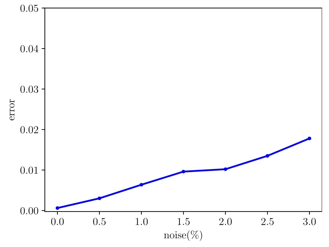
Figure 6.The comparison of the relative 2 errors of the prediction results under small perturbations with different noise levels.

Next,the performance of this framework in the presence of noise is compared.By adding some small amounts of noise

where δ denotes the amount of noise,s is the standard deviation of u(t,x)andwe disturb the data.From fgiure 6,the numerical experiments reveal that the architecture is remarkably robust for some small noise and then the model is able to perform the long-term prediction even when trained with noisy data.That is to say,the model could reconstruct the solution behavior from noisy data.From these experiments,we believe that the input noise at a certain extent can be regarded as a regularization mechanism that increases the robustness of the network.This is a kind of weak generalization.Additionally,this perturbation phenomenon can also be described by results on orbital stability and asymptotic stability of solitons[20,21]from the mathematical viewpoint.

As the noise level increases,however,the accuracy of the predicted solution decreases and the training time increases remarkably.Here,for noisy data,we can increase the numbers of training data to decrease the relative error and then improve the accuracy of the predicted solution.The experimental comparison of the influence of different numbers of sub-sampled data points on the prediction under different noise levels is given in table 2.

Generally speaking,with more layers and more neurons,the model has a better performance[22].So,we carry out a lot of numerical experiments in order to check this empirical result.See table 3 for the comparison with different numbers of hidden layers and neurons per hidden layer.Some more detailed theoretical analyses are also conducted[23,24].

Last,we also train the model using the Adam[25]optimizer with default parameter setups to approximate the antikink solution to the sine-Gordon equation.The training procedure takes approximately 2.5 h with Nu=100 and Nf=10 000 under 30 000 epochs.The relative2error between the exact and predicted solutions is 1.47e-02.The experimental result shows that the L-BFGS algorithm is much faster than Adam in this case and it gets a more accurate solution.However,the former sometimes suffers from some convergence issues.

Table 2.Relative2 errors for different numbers of data points under the distortion of different noise levels.

Table 2.Relative2 errors for different numbers of data points under the distortion of different noise levels.

Noise0%Noise1%NfNf Nu1000500010 00020 000Nu1000500010 00020 000 103.67e-01 1.47e-01 1.02e-01 2.27e-01105.17e-01 1.41e-01 8.58e-02 5.34e-02 506.98e-03 2.12e-03 1.14e-03 1.68e-03501.35e-02 5.71e-03 5.81e-03 3.75e-03 1002.91e-03 1.48e-03 1.37e-03 1.23e-031009.52e-03 5.95e-03 6.92e-03 3.55e-03 2001.07e-03 1.21e-03 9.73e-04 6.09e-042003.60e-03 1.42e-03 2.59e-03 2.03e-03

Table 3.Relative 2 errors for different numbers of hidden layers and neurons per hidden layer under a fixed random seed.

Table 3.Relative 2 errors for different numbers of hidden layers and neurons per hidden layer under a fixed random seed.

Neurons Hidden layers10204080 4 5.09e-01 7.01e-04 4.98e-04 1.21e-03 8 1.76e-03 1.47e-03 9.65e-04 8.43e-04 127.91e-04 7.87e-04 6.09e-04 7.05e-03 166.65e-04 3.38e-04 3.70e-04 2.16e-03

4.Conclusions and discussion

In this paper,we propose a new architecture that combines deep residual network with underlying physical laws for extracting soliton dynamics of the sine-Gordon equation from spatiotemporal data.This architecture can be used easily to train very deep networks and then alleviates the gradient exploding and vanishing problems.Moreover,we use the logcosh function rather than the square function in the objective in this paper in order to accelerate the training and improve the performance of the network.The numerical results show that the model could reconstruct the solution behaviors of the equation very accurately.Moreover,this model is remarkably robust under small disturbances to some extent.

Despite some progress,we are still at the early stages of understanding the capabilities and limitations of such deep learning models.In addition,other advanced frameworks,for example,generative adversarial networks,recurrent neural networks and networks with some numerical schemes embedded,will also be considered in the future research.

Acknowledgments

The first author would like to express his sincere thanks to Dr Yuqi Li and Dr Xiaoen Zhang for their valuable comments and excellent suggestions on this work.The authors gratefully acknowledge the support of the National Natural Science Foundation of China(Grant No.11675054),Shanghai Collaborative Innovation Center of Trustworthy Software for Internet of Things(Grant No.ZF1213)and Science and Technology Commission of Shanghai Municipality(Grant No.18dz2271000).