Evaluation of the China Ocean Reanalysis (CORA) in the South China Sea*

FAN Maoting , WANG Huizan , , ZHANG Weimin , , HAN Guijun , WANG Pinqiang

1 College of Meteorology and Oceanography, National University of Defense Technology, Changsha 410073, China

2 Key Laboratory of Software Engineering for Complex Systems, National University of Defense Technology, Changsha 410073, China

3 School of Marine Science and Technology, Tianjin University, Tianjin 300072, China

Abstract The daily regional reanalysis product of the China Ocean Reanalysis (CORA) product was released in website in 2018. Using in situ observational data including Argo profi ling fl oats, drifters, and cruise data, the performance of CORA in the South China Sea in terms of temperature, salinity, current and mixed layer depths is evaluated based on timescale (seasonal and interannual) and spatial distribution characteristics. The CORA temperature, salinity, and mixed layer depth show certain seasonal and interannual variations. In 50–400 m depth in the SCS, the CORA temperature is colder in winter and warmer in summer and autumn. In 0–150 m in the SCS, the CORA salinity is higher in most time of the year. However, in the second half of the year, the salinity is slightly weaker in 100–150 m depth. In most years, the CORA mixed layer depths tend to be shallower, and in season, shallower in winter and deeper in summer. In spatial distribution, the closer the area is to the coast, the greater the CORA errors would be. The CORA temperature is colder in the western side and warmer in the eastern side, resulting in a weaker SCS western boundary current (SCSwbc). In most areas, the CORA mixed layer depths are shallower. In the area close to the coast, the CORA mixed layer depths change rapidly, and the deviations in the mixed layer depths are larger. In the central SCS, the CORA mixed layer depths change slowly, and the deviations in the mixed layer depths are also small.

Keyword: China Ocean Reanalysis (CORA); South China Sea (SCS); drifter, Argo; cruise data; evaluation

1 INTRODUCTION

Multiscale ocean phenomena or processes can be described by ocean temperature, salinity, current, etc. Existing ocean in situ observations cannot easily meet the requirements of underwater marine environmental support due to sparse spatial and temporal distributions. Current ocean model simulations can provide some insights into ocean variability, but these simulations are aff ected by biases due to errors in model formulation, specifi cation of initial states and forcings. The high-resolution three-dimensional temperature, salinity and current reanalysis product can reproduce changes in the ocean state from past to present. Ocean reanalysis is based on the ocean dynamic model, using data assimilation techniques to assimilate multisource ocean historical observations into numerical models. The ocean state fi eld from the ocean reanalysis can refl ect the physical correlation of the ocean state changes, reproduce the characteristics of long-term timeseries and multiscale spatiotemporal variation, and provide accurate ocean background fi eld information for ocean numerical prediction and marine environmental protection. Therefore, ocean reanalysis products, such as Simple Ocean Data Assimilation (SODA) (Carton et al., 2000a, b), Estimating the Circulation and Climate of the Ocean (ECCO) (Stammer and Chassignet, 2000), Hybrid Coordinate Ocean Model (HYCOM) (Chassignet et al., 2007), Ocean ReAnalysis System 4 (ORAS4) (Balmaseda et al., 2013), Ocean ReAnalysis Pilot 5 (ORAP5) (Zuo et al., 2017) and China Ocean Reanalysis (CORA) (Han et al., 2011, 2013a, b), have been developed.

Due to the diff erences of observational data, numerical models, and data assimilation methods applied, various ocean reanalysis products are diff erent from each other in the ocean state reproduction capability (Wang et al., 2018b), and thus the product quality shall be evaluated. Wu et al. (2013) analyzed the seasonal and interannual variability in sea surface temperature (SST) in China seas based on CORA datasets. Balmaseda et al. (2013) evaluated ORAS4 based on observed ocean currents and sea-level gauges. Zuo et al. (2017) evaluated ORAP5 and showed that ORAP5 simulation have improved in the northern extratropics (especially for salinity). Balmaseda et al. (2015) exploited the diversity of existing ocean reanalysis for the Ocean Reanalysis Intercomparison Project (ORA-IP). Karspeck et al. (2017) analyzed the mean and variability of the Atlantic meridional overturning circulation as represented in six ocean reanalysis products. However, available reanalysis products are evaluated for the global ocean and large-scale features. The evaluation of the special marine environment adaptability in the off shore area is often insuffi cient (Zhang et al., 2016a). As the largest marginal sea in China, the South China Sea (SCS) is susceptible to topography, monsoon, and the Kuroshio activity. The spatial and temporal distribution characteristics of temperature, salinity, and current are complex, regional characteristics are obvious, multiscale ocean phenomena and processes are rich, and there is a large diff erence in the SCS from the open ocean (Zeng et al., 2014). For use in off shore China, such as the SCS, the abovementioned reanalysis products often show large diff erences when describing China’s marginal ocean, which is related to the diff erent models, assimilation methods, and observational data used in the diff erent reanalysis products.

In 2009, a trial version of the regional ocean reanalysis for the coastal waters of China and adjacent seas, known as CORA Version Trial, was released by the National Marine Data and Information Service of China (NMDIS). In 2013, CORA version 1.0 was produced, which included a global ocean reanalysis and improved regional ocean reanalysis. In 2018, the daily and monthly regional reanalysis product and monthly global reanalysis product were released. CORA is the reanalysis product with the highest spatial and temporal resolutions released in China. To better protect the marine environment in the SCS and reproduce the current fi eld and temperature and salinity structure, it is urgent to evaluate the new generation of Northwestern Pacifi c long-term highresolution ocean reanalysis products.

To eff ectively evaluate the performance of the daily product in the SCS, based on in situ observational data such as Argo, drifters and cruise data, the performance of CORA in the SCS in terms of temperature, salinity, current and mixed layer depths based on the timescale (seasonal and interannual) and spatial distribution characteristics are evaluated. This article is organized as follows. The data are described in Section 2. A preliminary evaluation of CORA based on observational data is presented in Section 3. The conclusion and discussion are presented in Section 4.

2 DATA

Four sources of data are used in this study: CORA datasets, Argo datasets, drifter datasets, and cruise data. The specifi cs of each dataset are as follows.

2.1 CORA datasets

The CORA datasets are derived from the daily average product of the regional ocean reanalysis system for the Northwestern Pacifi c, which is publicly released by NMDIS. The ocean model used in CORA is a parallel version of the Princeton Ocean Model with a generalized coordinate system (POMgcs) developed by NMDIS. Both wave-induced mixing and tide-induced mixing are considered in the POMgcs to improve the accuracy of coastal waters in China. NCEP Reanalysis is employed as the atmospheric forcing for regional ocean reanalysis systems. Oceanic observations assimilated into regional ocean reanalysis systems include in situ temperature/salinity profi les from NMDIS archive, World Ocean Database 2009 (WOD09), Global Temperature and Salinity Profi le Project (GTSPP), and Argo project, sea level anomalies (SLA) from TOPEX/POSEIDON (T/P), Jason-1, ERS-2 and ENVISAT, and SST from the Reynolds SST dataset (Han et al., 2013a). The product area coverage is 99°E–150°E, 10°S–52°N. A horizontal C-grid has a 0.5°×0.5° horizontal resolution telescoping to 0.25° meridional spacing in the tropical region, and the total horizontal grid number is 720×348, the z-level standard vertical grid is used in CORA model, with a total of 35 vertical levels for confi guration (Han et al., 2013a). CORA data is downloaded from http://cora.nmdis.org.cn/. The minimum and maximum water depth is 2.5 m and 5 500 m, respectively. The temporal resolution is daily. The dataset storage format is a binary fi le. In this study, SCS region (100°E–125°E, 0°N–25°N) datasets from 2007–2017 are mainly used.

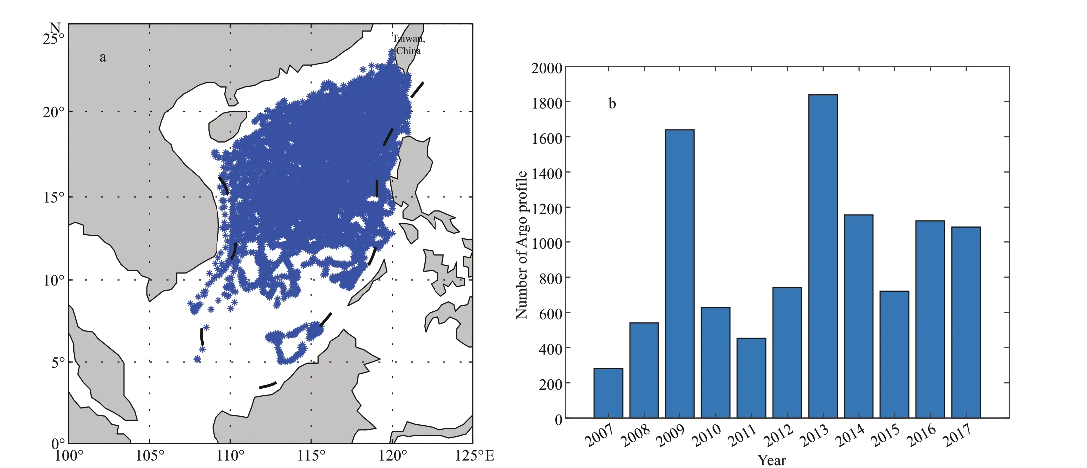
Fig.1 Positions of Argo profi les from 2007-2017 in the SCS (a) and the number of Argo profi les in the SCS from 2007-2017 (b)

2.2 Argo datasets

Argo is a global array of approximately 4 000 freedrift profi le fl oats used to measure data such as temperature and salinity of the upper 2 000 m of the ocean. The broad-scale global array of temperature/salinity profi ling fl oats, known as Argo, has already grown to be a major component of the ocean observational system. Argo is a standard to which other developing ocean observing systems can be compared. In this study, globally quality-controlled temperature/salinity datasets from Argo profi ling fl oats are used (Wang et al., 2012). The Argo datasets (downloaded from ftp://ftp.argo.org.cn/pub/ARGO/global/) in the SCS from 2007–2017 are selected. Figure 1a shows the distribution of the Argo profi les in the SCS from 2007–2017, and Fig.1b shows the number of Argo profi les in the SCS from 2007–2017. The Argo fl oats in the SCS are mainly distributed in deep water depths north of 8°N. The annual average number of Argo profi les is 927. There are some diff erences in the number of diff erent years, but all are more than 280. The largest number of profi les occurred in 2013 and was 1 838.

2.3 Drifter datasets

NOAA’s Global Drifter Program (GDP) has deployed more than 25 000 drifters since the program began in 1979. The drifter is a surface drifting buoy that refl ects the ocean current fi eld information as the seawater moves. The drifter consists of a surface buoy and a subsurface drogue (sea anchor) attached by a long, thin tether. The buoy measures temperature and other properties and is equipped with a transmitter to send the data to passing satellites. The drogue dominates the total area of the instrument and is centered at a depth of 15 m beneath the sea surface. Thus, the drifter buoy refl ects the fl ow fi eld at a depth of 15 m. The drifter datasets (downloaded from https://www.aoml.noaa.gov/phod/gdp/index.php) used in this study are SCS data from 2007–2017, with approximately 110 000 data points. Figure 2 shows the positions of the drifters that are widely distributed in the SCS.

2.4 Cruise data in the SCS

In this study, cruise data were provided by South China Sea Institute of Oceanology, Chinese Academy of Sciences. These data have not been assimilated into CORA. Therefore, they are independent in situ observational data. From 2014 to 2017, four cruises were conducted in research vessels in the SCS (Table 1). Each cruise visited 10 observation stations. CTD (conductivity-temperature-depth) used in these cruises was SBE 911Plus CTD.

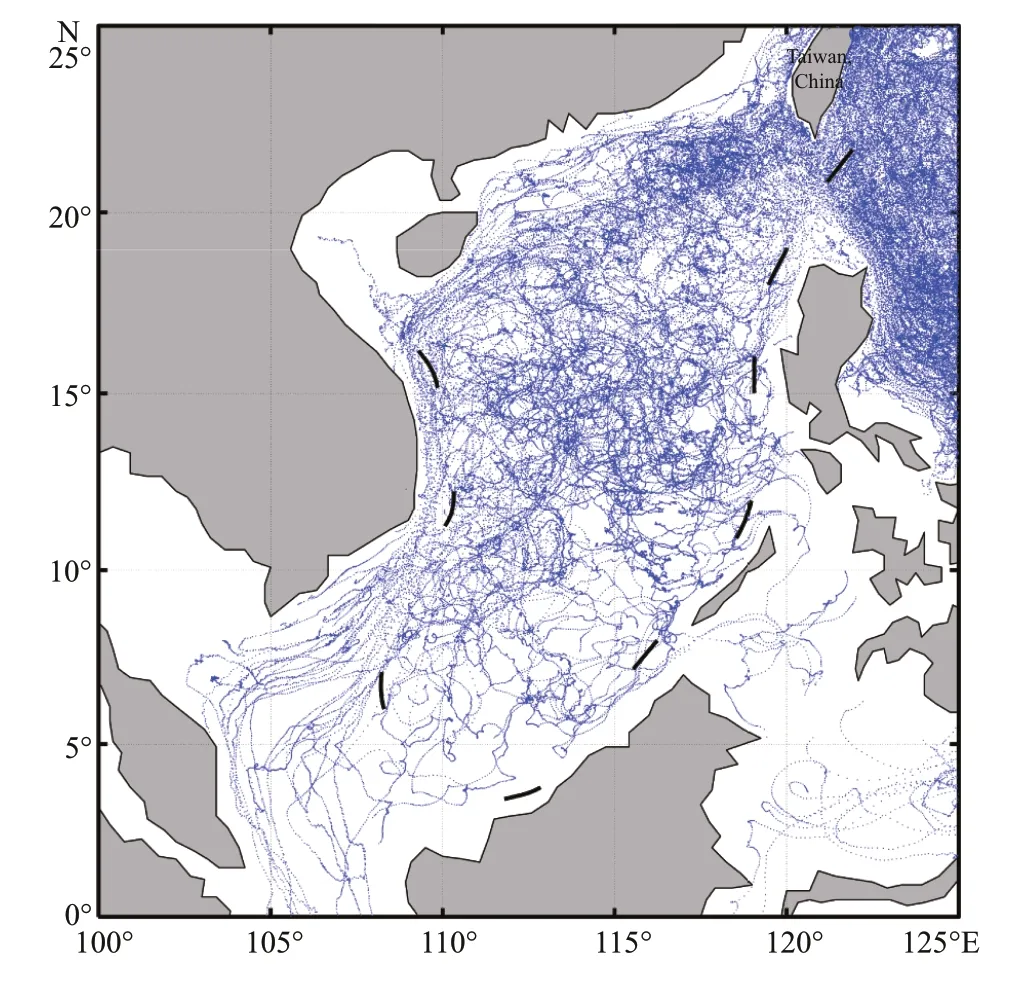
Fig.2 Traces of drifters in the SCS from 2007-2017

3 PRELIMINARY EVALUATION OF CORA BASED ON OBSERVATIONAL DATA

Due to the scarcity of in situ observations in the SCS, the current quality inspection and evaluation of reanalysis products in the SCS is diffi cult and contains uncertainty. To evaluate the performance of CORA in the SCS, the temperature, salinity, current, and mixed layer depth errors from the time variation scale (seasonal and interannual) and spatial distribution characteristics were evaluated. The Argo profi ling fl oats, drifters and cruise data are the three most important sources of in situ observational data. The quality-controlled Argo profi ling datasets (Wang et al., 2012) and cruise data were used to evaluate the temperature, salinity, and mixed layer depth errors in CORA. The quality-controlled drifters (Lumpkin et al., 2012) were used to evaluate the surface current of CORA at a depth of 15 m.

3.1 Seasonal and interannual variation characteristics of the CORA errors

Seasonal and interannual feature error evaluations mainly analyze the CORA temperature, salinity and mixed layer depth errors in the SCS over time to evaluate whether the CORA errors experience specifi c seasonal or annual changes. The specifi c method is as follows.

Thirty-fi ve standard layers are chosen with depths of 2.5, 10, 20, 30, 50, 75, 100, 125, 150, 175, 200, 225, 250, 275, 300, 325, 350, 375, 400, 425, 450, 500,550, 600, 700, 800, 900, 1 000, 1 100, 1 200, 1 300, 1 400, 1 500, 1 750, and 2 000 m. The CORA data are interpolated to the coordinate point where the Argo observational data are located, and the temperature and salinity deviations of CORA and Argo, the average deviations and the root mean square errors are calculated in each standard layer.

Table 1 Description of cruise data in the SCS

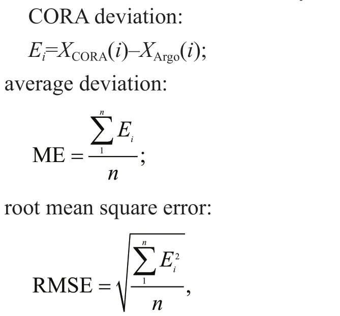
whereXArgo(i) is the temperature or salinity data of theithArgo profi le in the standard layer, andXCORA(i) is the CORA temperature or salinity data corresponding to the Argo position in the standard layer. In addition,Ei(i=1, 2, ...,n) is the error of theithCORA data in the standard layer, andnis the number of Argo profi les corresponding to the comparison.

Figure 3 is an example of the CORA temperature and salinity deviations in the SCS in Jan. 2017, which also shows the monthly mean deviations and root mean square errors. Figure 3a & b is the sets of CORA temperature and salinity deviations corresponding to all Argo profi les in the SCS in Jan. 2017, and Fig.3c & d is the mean deviations and root mean square errors, respectively, of all corresponding profi les. For a total of 132 months from 2007–2017, a similar picture can be drawn for each month.

To evaluate the CORA temperature and salinity errors with seasonal and interannual performances, based on the 132 monthly CORA temperature and salinity errors obtained above, the monthly average temperature and salinity errors (Fig.4a & b), average errors of the same month for many years (Fig.4c & d) and annual mean errors (Fig.4e & f) from Jan. 2007 to Dec. 2017 were calculated and plotted.

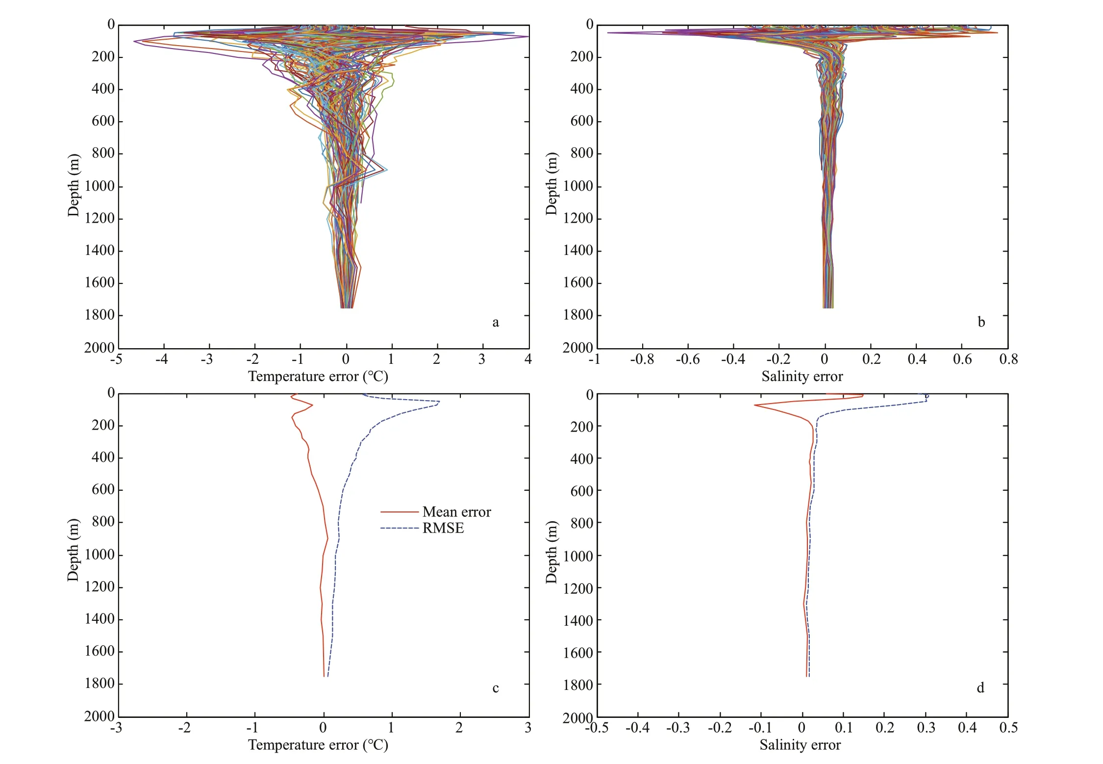
Fig.3 Temperature deviations (CORA minus Argo) (a), salinity deviations (CORA minus Argo) (b), monthly mean deviations and root mean square errors of CORA temperature (c), and monthly mean deviations and root mean square errors of CORA salinity (d) in Jan. 2017 in the SCS

First, we examine the characteristics of the ocean temperature errors. Figure 4a shows that at depths of 50–400 m, the CORA temperature error is nearly alternately colder and warmer, which is especially evident after 2013. Figure 4c shows that at depths of 50–400 m, the CORA temperature error varies seasonally in the SCS. The temperature is colder in winter (Jan., Feb., and Dec.), and the coldest temperature occurs in Jan. In summer and autumn (May to Nov.), the temperature is warmer, and the warmest temperature occurs in Jul. In spring (Mar. and Apr.), the temperature errors are small. From Apr. forward, the temperature gradually warmed from the near surface layer, and the deepest warm range in Sep. reached approximately 500 m and then gradually decreased. Based on the annual deviations shown in Fig.4e, the annual average deviations can be divided into three parts: from 2007–2009, the temperature is warmer at depths of 50–200 m, and the temperature it is colder at depths of 300–1 000 m. The temperature deviations from 2009–2012 are generally small. From 2012–2017, the temperature is colder at depths of 0–50 m and warmer overall at depths of 50–500 m, which is the most obvious in 2015.

Next, the characteristics of the salinity errors are checked. Figure 4b shows that the most signifi cant depth of the salinity deviations occurs between 0 m and 200 m. The monthly variation in the errors in Figure 4d shows that the CORA salinity is higher during most months from 0 m to 150 m. However, the variations are weak at depths of 100 m to 150 m during the second half year (Jul. to Dec.). As shown in Fig.4f, at depths of 0 m to 150 m, the salinity is higher from 2007–2015, while the salinity is lower in 2016–2017. In addition, the salinity at depths deeper than 150 m is slightly higher from 2008–2011.

As shown in Fig.4a, b, e & f, the CORA temperature and salinity errors are generally small from 2009–2012. In 2008 and 2014, the temperature between 50 m and 200 m reached a warm peak, and the salinity peaked at depths of 0 m to 50 m.

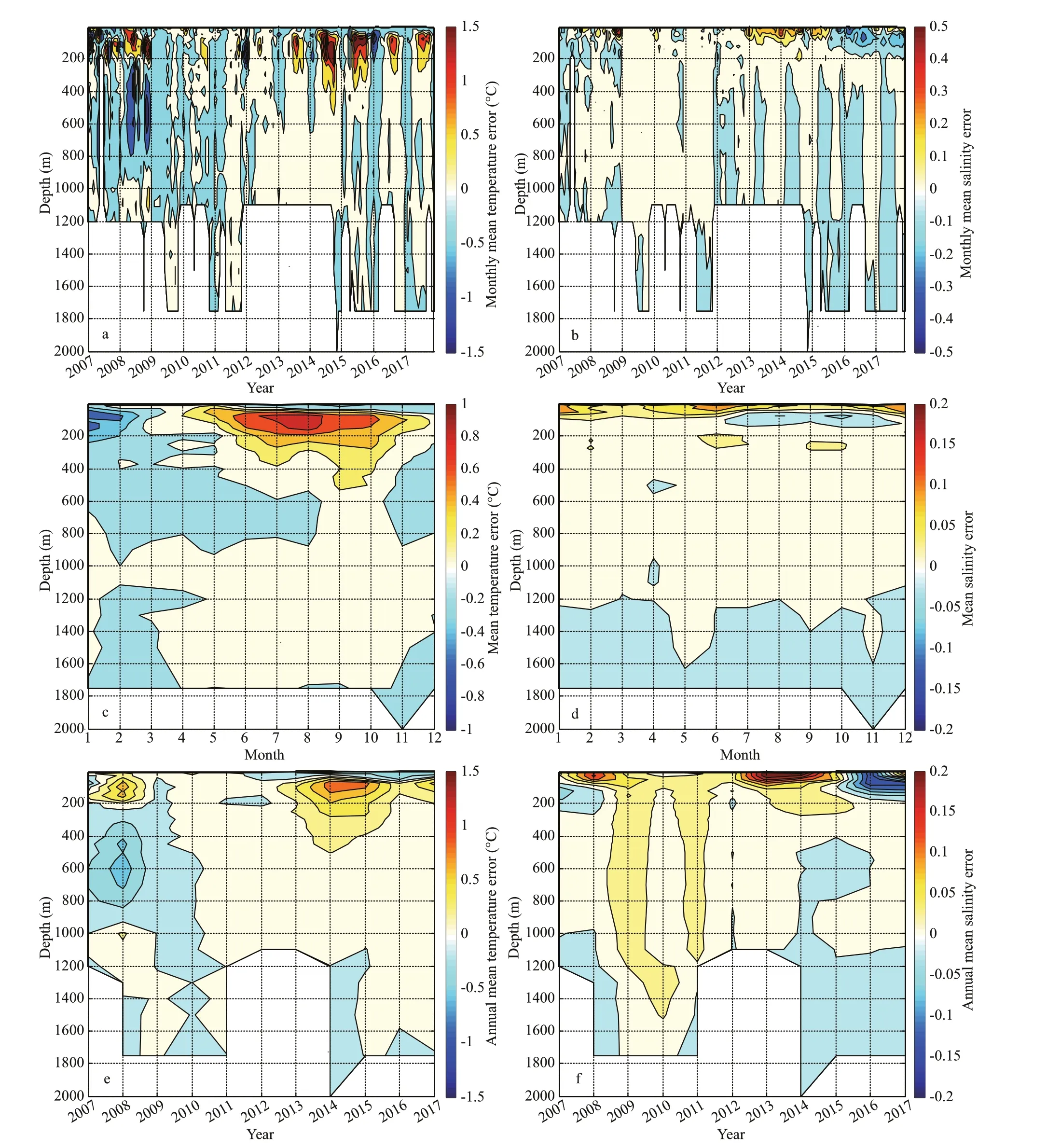
Fig.4 Monthly mean errors of CORA temperature (a), monthly mean errors of CORA salinity (b), mean errors of CORA temperature for the same month over many years (c), mean errors of CORA salinity for the same month over many years (d), annual mean errors of CORA temperature (e), and annual mean errors of CORA salinity (f) from Jan. 2007 to Dec. 2017 in the SCS

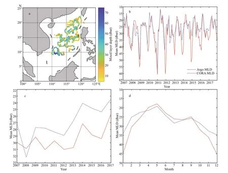
Fig.5 In the SCS, density mixed layer depths of CORA in 2016 (a), monthly average mixed layer depth comparison chart of CORA and Argo from Jan. 2007 to Dec. 2017 (b), annual average mixed layer depth comparison chart of CORA and Argo from 2007 to 2017 (c), monthly average mixed layer depth comparison chart of CORA and Argo for the same month over many years (d)

To better understand the comprehensive bias eff ect of the temperature and salinity vertical distributions, the mixed layer depths are used for evaluation. Using Holte and Talley’s (2009) mixed layer depth calculation method, which off ers a clear improvement in the accuracy of mixed layer depth, the density mixed layer depth of each Argo profi le can be determined by the Argo temperature, salinity, pressure and other data. In this study, Argo original profi ling observations (not standard layers) are used to calculate the Argo mixed layer depths. They have a relatively high vertical resolution at depths of 0–100 m. When CORA mixed layer depths were calculated, CORA data was interpolated to Argo original profi ling observations, which ensured that CORA also had a relatively high vertical resolution in the upper ocean. Taking 2016 as an example, the CORA temperature and salinity were interpolated to the position where Argo was located, and the CORA density mixed layer depth at this location could be calculated. Figure 5a shows the CORA density mixed layer depths at the Argo profi le locations in the SCS in 2016. The monthly average mixed layer depths (Fig.5b), the annual average mixed layer depths (Fig.5c), and the average mixed layer depths for the same month over many years (Fig.5d) can be calculated.

Figure 5b shows that the CORA mixed layer depths are the same as those of Argo, but the variation amplitude is diff erent. The amplitude of the mixed layer depths refl ected by Argo is slightly larger than that of CORA. Figure 5c refl ects that the CORA mixed layer depths are shallower during most years, and there is a tendency to become shallower every year. Figure 5d shows that the mixed layer depths in winter are deep, reaching the deepest valley in Dec. and Jan., the shallow depths of the mixed layer occur in summer, and the shallowest peak is in May. The CORA errors for the mixed layer depths show the seasonal variation characteristics, which are shallower in winter and deeper in summer compared to the Argo observations.

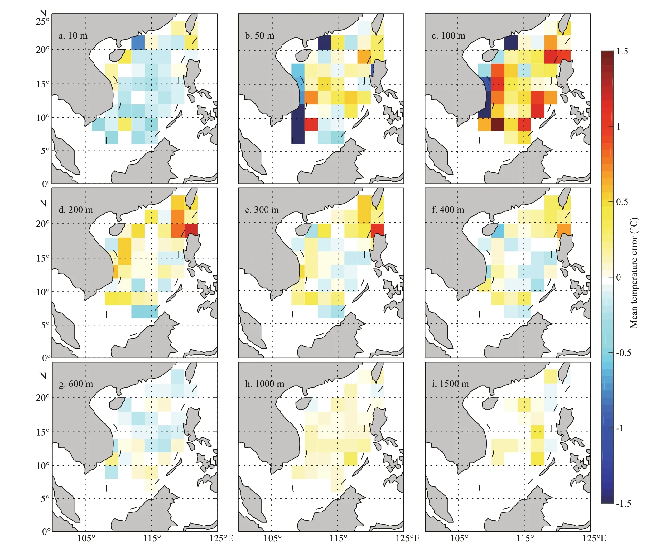
Fig.6 Mean deviations in CORA temperature at diff erent depths in the same grid in the SCS over many years

The mixed layer depth is related to SST and subsurface temperature. In most areas of the northwestern Pacifi c, SST has a negative correlation with mixed layer depth, and subsurface temperature has a positive correlation with mixed layer depth (Wang et al., 2018a). As the SST of CORA shown in Fig.4a & c is slightly colder, the surface errors are small. The subsurface temperature of CORA is obviously warmer in summer and colder in winter, which is related to the seasonal variations of CORA mixed layer depths, i.e., shallower in winter and deeper in summer (Fig.5d).

In summary, the temperature, salinity, and mixed layer depth errors of CORA show certain seasonal and interannual variations.

3.2 Spatial distribution characteristics of CORA errors

To study the distribution characteristics of CORA errors at diff erent positions, the SCS area is meshed, and the CORA temperature, salinity, and mixed layer depth errors in diff erent grids are analyzed to evaluate whether the CORA errors are related to the spatial position. The specifi c steps are as follows.

The SCS area was divided by a 2°×2° grid to obtain a grid of size 13×13. In diff erent grids, CORA is interpolated to the coordinate points of all Argo data in the grid, and the CORA temperature, salinity deviations, mean deviations and root mean square errors are calculated in the standard layer. The calculation method and formulas are the same as those in Section 3.1 and are not detail here. Based on the CORA temperature and salinity errors in the diff erent meshes obtained above, the average deviations in CORA temperature and salinity in the same grid over many years were calculated in diff erent standard layers.

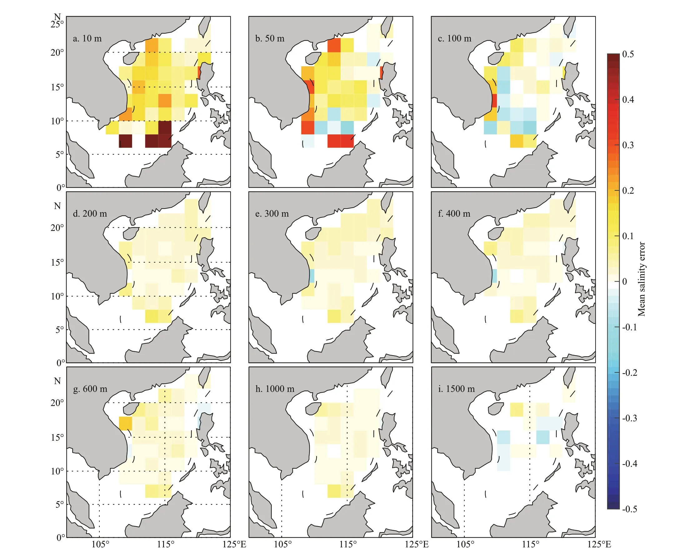
Fig.7 Average deviations in CORA salinity at diff erent depths in the same grid in the SCS over many years

Figure 6 shows the average temperature deviations in CORA at diff erent depths in the same grid over the years in the SCS. As seen in Fig.6, the temperature deviations are obvious at depths of 50–200 m (Fig.6b, c & d), and the temperature deviations are small below 1 000 m depth (Fig.6h & i). The temperature deviations in CORA are obviously colder at depths of 50–100 m on the west and northwest sides of the SCS (Fig.6b & c). At a depth of 100 m near the Luzon Strait and the northern side of Palawan, the temperature deviation is warmer (Fig.6c).

Figure 7 shows the average deviations in salinity at diff erent depths in CORA in the SCS over many years. As seen in Fig.7, the salinity deviations are obvious at depths of 10–100 m (Fig.7a, b & c), and the salinity errors are smaller below a depth of 200 m (Fig.7d, e, f, g, h & i). At depths of 10–50 m in the west and south edges of the SCS, the CORA salinity is obviously higher (Fig.7a & b).

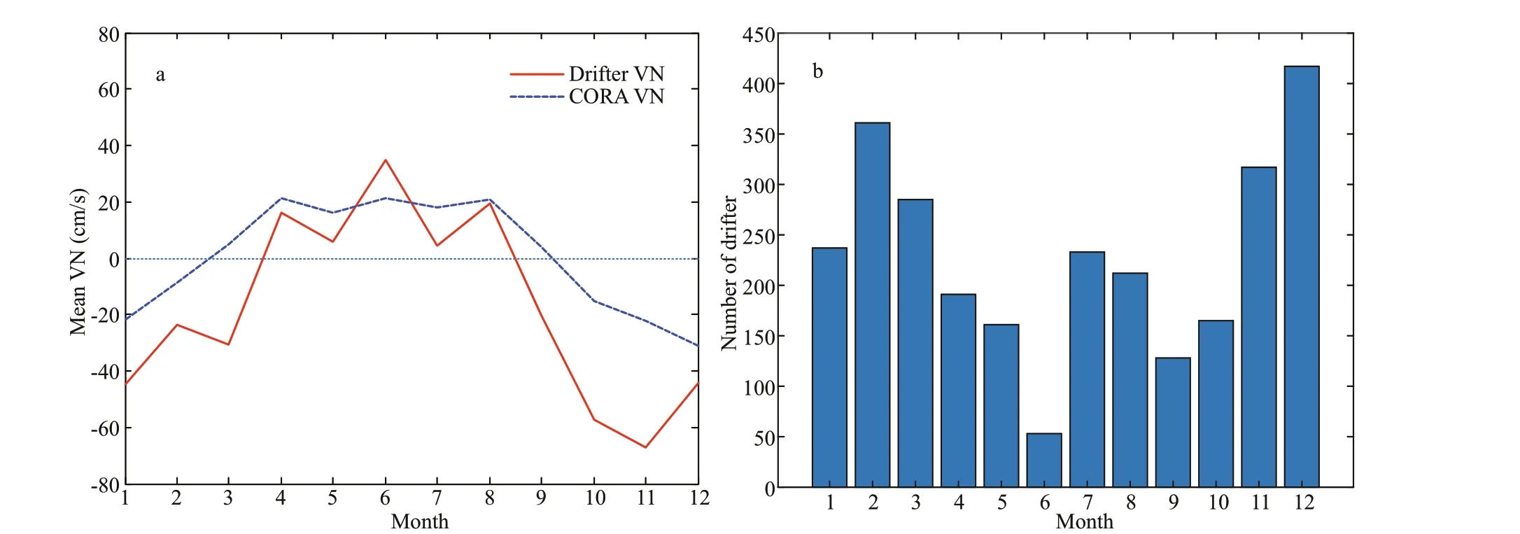
Fig.8 The SCSwbc (108°E-111°E, 10°N-15°N) from 2007 to 2017: the average meridional velocity of the CORA surface current and the average meridional velocity of the drifter’s current (a), and the drifter’s number of diff erent months (b)

Figure 6 also shows that at depths of 50–100 m (Fig.6b & c), a region with signifi cant temperature errors appears in the SCS east of Vietnam (108°E–111°E, 10°N–15°N), and the temperature on the west side (108°E–110°E) is obviously colder, and the temperature is obviously warmer on the east side (110°E–111°E). This is the location of the SCS western boundary current (SCSwbc). The SCSwbc fl ows northward in the summer and southward in the winter, and the fl ow in winter is stronger than that in summer (Xu et al., 2013; Zhang et al., 2016b). To determine whether the signifi cant area of these temperature errors is related to the strength of the simulated SCSwbc in CORA, the average meridional velocity of the CORA surface current in this area is compared with the average meridional velocity of the drifter’s current. CORA surface current is at depths of 2.5, 10, 20, 30, 50, 75, 100 m, etc. In this study, Akima interpolation algorithm was used to calculate the fl ow fi eld of CORA at a depth of 15 m before comparing it with drifter fl ow fi eld, which is also at a depth of 15 m. The number of diff erent months for the drifter in this region is shown in Fig.8b. The SCSwbc of the CORA surface simulation is normal in summer and weak in winter (Fig.8a). Because the SCSwbc is dominated by the geostrophic current, according to the calculation formula of the geostrophic current, the geostrophic current is mainly related to density, and the density is mainly controlled by temperature. The temperature simulated in CORA and shown in Fig.6 is colder on the west side and warmer on the east side, resulting in a weaker SCSwbc, which is consistent with the SCSwbc characteristics shown in Fig.8.

In diff erent grids, the mixed layer depths of all CORA profi les are calculated. The computing method is the same as that used in Section 3.1. The average mixed layer depths in all grids were determined (Fig.9, contour). Taking the average mixed layer depths of Argo as a standard reference, the average mixed layer depth errors of CORA are determined (Fig.9, color, CORA minus Argo).

Figure 9 shows that in the area close to the coast, the CORA mixed layer depths are shallower. On the west and south sides of the SCS, CORA shows the shallowest depths of the mixed layer. In the central SCS, the CORA mixed layer depths are deeper. Figure 9 also shows that the CORA mixed layer depths in most grids are shallower than the actual Argo observations. In the area close to the coast, the contour graph of the CORA mixed layer depths is dense, the CORA mixed layer depths change rapidly, and the deviations in the mixed layer depths are larger. In the central SCS, the contour graph of the CORA mixed layer depths is sparse, the CORA mixed layer depths change slowly, and the deviations in the mixed layer depths are also small.

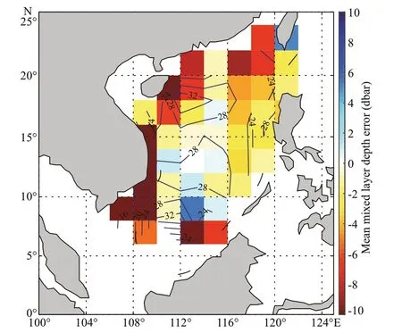
Fig.9 Mean mixed layer depth errors of CORA (color, CORA minus Argo) and mean mixed layer depths of CORA (contour)

In summary, considering the spatial distribution characteristics, the areas with large temperature, salinity and mixed layer depth errors are usually in the grid near the coast, while in the central SCS, the errors are relatively small, which means that the closer the location is to the coast, the greater the CORA errors will be. The temperature structure simulated in CORA is colder on the west side and warmer on the east side, resulting in a weaker SCSwbc.

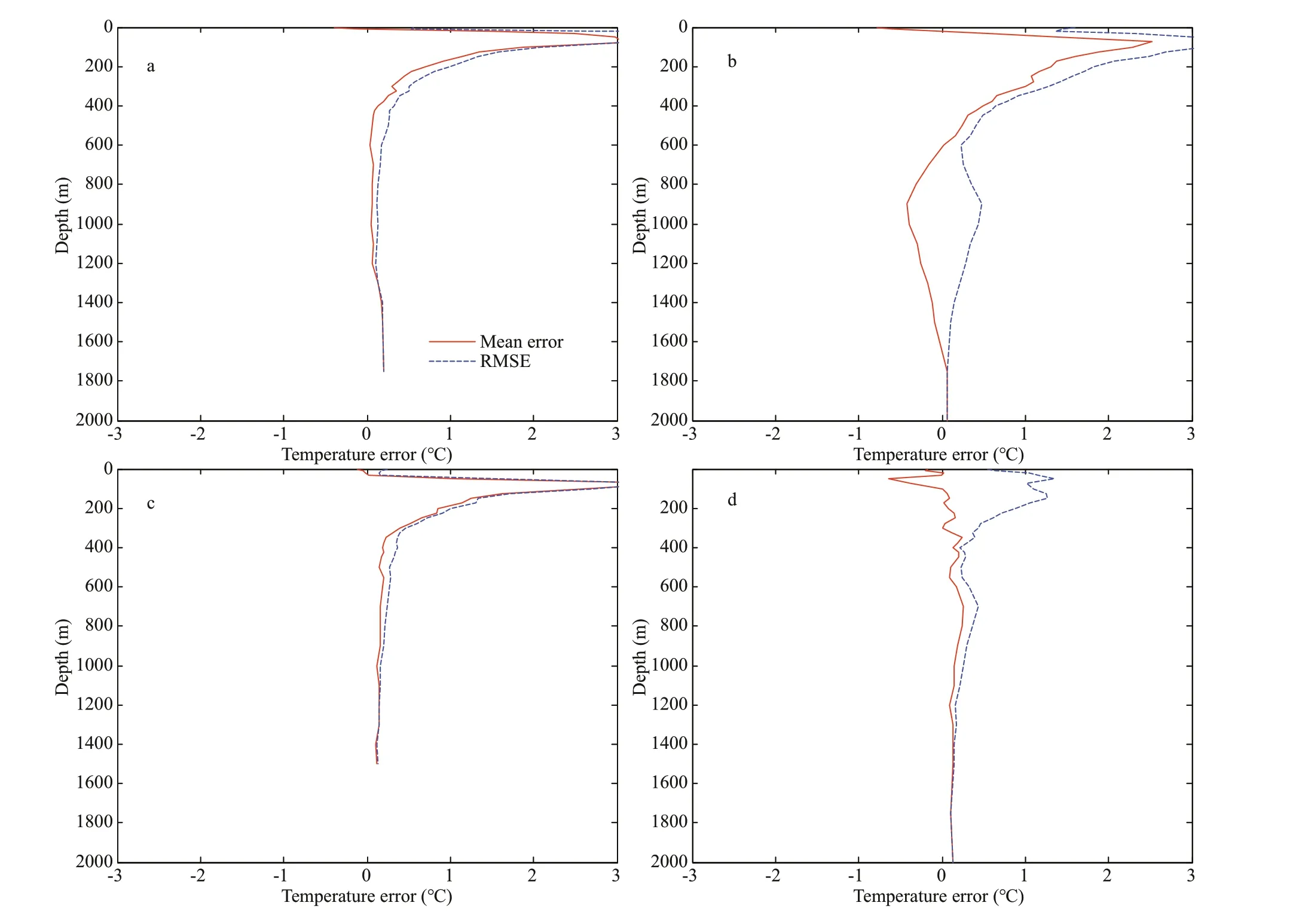
Fig.10 Mean errors (CORA minus CTD) and root mean square errors of CORA temperature in Sep. 2014 (a), Jul. 2015 (b), Sep. 2015 (c), and Apr. 2017 (d)

3.3 Evaluation of CORA based on cruise data in the SCS

Based on these cruise data (CTD represents cruise data in this paper) in the SCS, the average errors and root mean square errors of CORA temperature and salinity can be obtained (Figs.10 & 11). The calculation method and formulas are similar to those in Section 3.1. Figure 10 shows that at depths of 50–400 m, the CORA temperature is warmer in Sep. 2014 (Fig.10a), Jul. 2015 (Fig.10b) and Sep. 2015 (Fig.10c). In Apr. 2017 (Fig.10d), the CORA temperature errors are small. This is consistent with the conclusions of CORA temperature error in Section 3.1 (Fig.4a & c).

As shown in Fig.11, at depths of 0–50 m, the CORA salinity is higher in Jul. 2015 (Fig.11b), Sep. 2015 (Fig.11c), and Apr. 2017 (Fig.11d). While at depths of 50–150 m, the CORA salinity is lower in Sep. 2014 (Fig.11a), Jul. 2015 (Fig.11b), Sep. 2015 (Fig.11c) and Apr. 2017 (Fig.11d). This is approximately consistent with the conclusions ofCORA salinity error in Section 3.1 (Fig.4b & d).

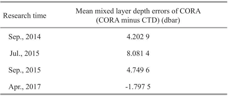
Table 2 Mean mixed layer depth errors of CORA compared to cruise data in the SCS

We also checked the mixed layer depths of CORA and CTD. The computing method is the same as that used in Section 3.1. Figure 12 shows the mixed layer depths of cruise data. Table 2 is mean mixed layer depth errors (CORA minus CTD) of CORA compared to cruise data in the SCS. It shows that mixed layer depths are shallower in Apr. and deeper in Jul. and Sep. This is also consistent with the conclusions of CORA mixed layer depth error in Section 3.1 (Fig.5d).

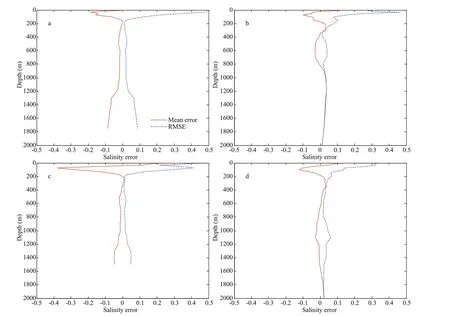
Fig.11 Mean errors (CORA minus CTD) and root mean square errors of CORA salinity in Sep. 2014 (a), Jul. 2015 (b), Sep. 2015 (c), and Apr. 2017 (d)

4 SUMMARY AND DISCUSSION

In this study, the temperature, salinity, current and mixed layer depth errors from the time variation scale (seasonal and interannual) and spatial distribution characteristics are evaluated. From the time variation scale, the CORA temperature, salinity, and mixed layer depth errors show certain seasonal and interannual variations. The cruise data validates these conclusions. At depths of 50 m to 400 m in the SCS, the CORA temperature is colder in winter and warmer in summer and autumn. The annual average deviations in the CORA temperature can be divided into three parts: from 2007 to 2009, the temperature is warmer at depths of 50 m to 200 m and colder at depths of 300 m to 1 000 m. From 2009 to 2012, the temperature deviations are generally small. From 2012 to 2017, the temperature is colder at depths of 0 m to 50 m and warmer overall at depths of 50 m to 500 m, which is most obvious in 2015. At depths of 0 m to 150 m in the SCS, the CORA salinity is higher during most months. However, during the second half of the year, the salinity is slightly weaker at depths of 100 m to 150 m. In most years, the CORA mixed layer depths are shallower and tend to become shallower every year. The CORA mixed layer depths show seasonal variation characteristics, which are shallower in winter and deeper in summer. In addition, this is related to the seasonal variations of subsurface temperature of CORA.

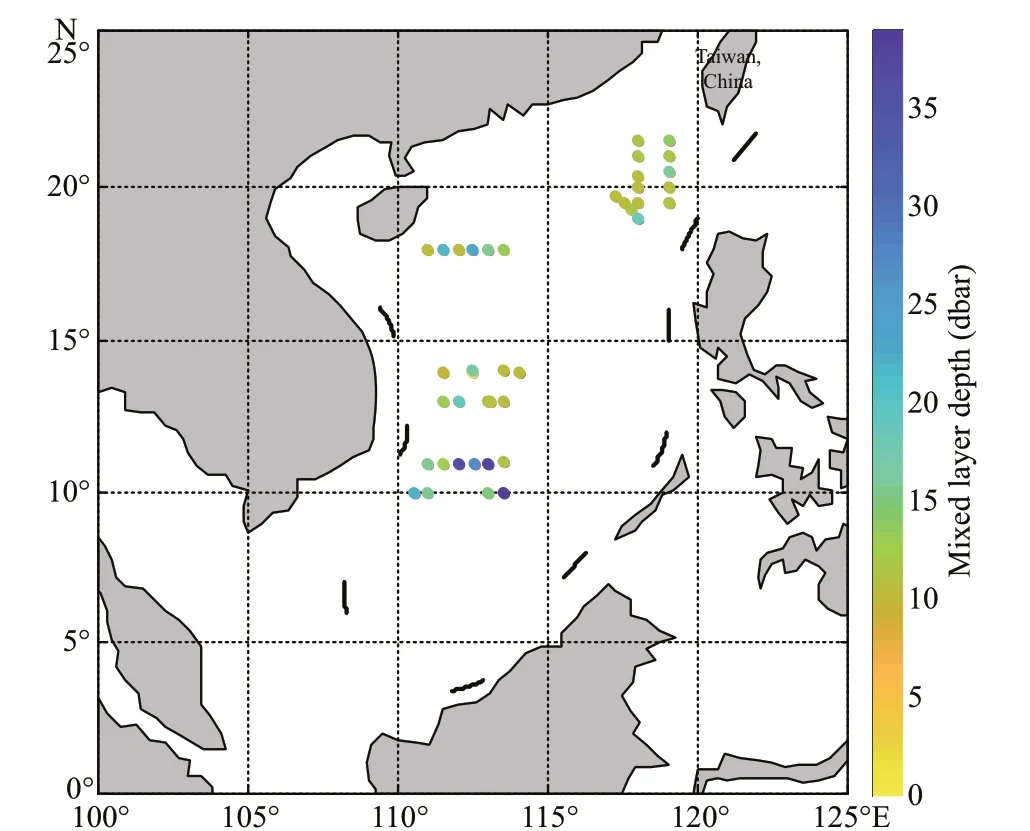
Fig.12 Mixed layer depths of cruise data in the SCS

From the spatial distribution characteristics, the areas with high temperature, salinity and mixed layer depth errors are usually in the area close to the coast, while in the central SCS, the errors are relatively small, which means that the closer the location is to the coast, the greater the CORA errors will be. The temperature structure simulated in CORA is colder on the west side and warmer on the east side, resulting in a weaker SCSwbc. At depths of 50 m to 200 m, the temperature deviations are obvious. Below depths of 1 000 m, the temperature deviations are small. At depths of 50–100 m on the west and northwest sides of the SCS, the CORA temperature is obviously colder. At a depth of 100 m, on the north side of Palawan and near the Luzon Strait, the temperature is warmer. At depths of 10–100 m, the salinity deviations are obvious. Below 200 m depth, the salinity errors are small. At depths of 10–50 m on the west and south edges of the SCS, the CORA salinity is obviously higher. In most areas, the mixed layer depths of CORA are shallower than the actual Argo observations. In the area close to the coast, the CORA mixed layer depths change rapidly, and the deviations in the mixed layer depths are larger. In the central SCS, the CORA mixed layer depths change slowly, and the deviations in the mixed layer depths are also small.

There are three main sources of CORA errors. First, it is obvious that the main source of errors is from the insuffi ciency of necessary temperature and salinity profi le observations in the SCS. Second, due to the limitation of POMgcs ocean model and computer conditions used for CORA, the model resolution is relatively low, and some small and medium-scale ocean processes are neglected. The CORA salinity is higher in the upper ocean because the freshwater fl ux is ignored in the ocean model. In addition, vertical mixing parameterization scheme also has an important eff ect on modeling the upper layer structure of temperature (Zhang et al., 2014). In the model used for CORA, the unperfect vertical mixing parameterization scheme may cause seasonal mixed layer depth errors. Subsurface temperature has a positive correlation with mixed layer depth in most areas of the northwestern Pacifi c (Wang et al., 2018a). This may be an important reason for the seasonal error of CORA temperature, i.e., colder in winter and warmer in summer and autumn. Last but not least, the third source of errors is from ocean data assimilation algorithms. The ocean data assimilation algorithm used for CORA is a three-dimensional variational analysis scheme designed within the multi-grid framework. The three-dimensional fi rst-guess fi eld used for the three-dimensional variational data assimilation of in situ temperature/salinity data is based on dynamic climatology, which stores the regression relationships, obtained from archives of historical temperature and salinity profi les, between subsurface temperature with sea surface height anomaly and SST. Because historical temperature and salinity profi les for the regression relationships are sparse and the number of data varies with the seasons and years, the three-dimensional fi rst-guess fi eld derived from regression relationships has certain seasonal and interannual variations, which may lead to corresponding seasonal and interannual variations of CORA errors.

In summary, by initially assessing the CORA performance in the SCS, CORA can basically refl ect the actual circumstances in the SCS, but there are still some aspects that can be improved. Using more ocean observational data can improve CORA accuracy, such as assimilation of drifter data into the model, which will improve the accuracy of the SCSwbc in the model. Additionally, improvements in model resolution and ocean data assimilation algorithms are very useful for reducing errors.

5 DATA AVAILABILITY STATEMENT

The datasets generated during and/or analyzed during the current study are available from the corresponding author on reasonable request.

6 ACKNOWLEDGMENT

We are grateful to the National Marine Data and Information Service of China (NMDIS) for developing, maintaining and making available (http://cora.nmdis.org.cn/) the CORA datasets that were used in this study. Argo data are from the China Argo Real-time Data Center (ftp://ftp.argo.org.cn/pub/ARGO/global/). Drifter data are from the National Oceanic and Atmospheric Administration Atlantic Oceanographic and Meteorological Laboratory Physical Oceanography Division (https://www.aoml.noaa.gov/phod/gdp/index.php). We thank the crew of research vessels (ExperimentNo.1&ExperimentNo.3) and all participants in the cruise for their eff orts in fi eld work.

References

Balmaseda M A, Hernandez F, Storto A, Palmer M D, Alves O, Shi L, Smith G C, Toyoda T, Valdivieso M, Barnier B, Behringer D, Boyer T, Chang Y S, Chepurin G A, Ferry N, Forget G, Fujii Y, Good S, Guinehut S, Haines K, Ishikawa Y, Keeley S, Köhl A, Lee T, Martin M J, Masina S, Masuda S, Meyssignac B, Mogensen K, Parent L, Peterson K A, Tang Y M, Yin Y, Vernieres G, Wang X, Waters J, Wedd R, Wang O, Xue Y, Chevallier M, Lemieux J F, Dupont F, Kuragano T, Kamachi M, Awaji T, Caltabiano A, Wilmer-Becker K, Gaillard F. 2015. The ocean reanalyses intercomparison project (ORA-IP).JournalofOperationalOceanography, 8(S1): s80-s97.

Balmaseda M A, Mogensen K, Weaver A T. 2013. Evaluation of the ECMWF ocean reanalysis system ORAS4.QuarterlyJournaloftheRoyalMeteorologicalSociety, 139(674): 1 132-1 161.

Carton J A, Chepurin G, Cao X H, Giese B. 2000a. A simple ocean data assimilation analysis of the global upper ocean 1950-95. Part I: methodology.JournalofPhysicalOceanography, 30(2): 294-309.

Carton J A, Chepurin G, Cao X H. 2000b. A simple ocean data assimilation analysis of the global upper ocean 1950-95. Part II: results.JournalofPhysicalOceanography, 30(2): 311-326.

Chassignet E P, Hurlburt H E, Smedstad O M, Halliwell G R, Hogan P J, Wallcraft A J, Baraille R, Bleck R. 2007. The HYCOM (hybrid coordinate ocean model) data assimilative system.JournalofMarineSystems, 65(1-4): 60-83.

Han G J, Fu H L, Zhang X F, Li W, Wu X R, Wang X D, Zhang L X. 2013a. A global ocean reanalysis product in the China Ocean Reanalysis (CORA) project.AdvancesinAtmosphericSciences, 30(6): 1 621-1 631.

Han G J, Li W, Zhang X F, Li D, He Z J, Wang X D, Wu X R, Yu T, Ma J R. 2011. A regional ocean reanalysis system for coastal waters of China and adjacent seas.AdvancesinAtmosphericSciences, 28(3): 682.

Han G J, Li W, Zhang X F, Wang X D, Wu X R, Fu H L, Zhang X S, Zhang L X, Li D. 2013b. A new version of regional ocean reanalysis for coastal waters of China and adjacent seas.AdvancesinAtmosphericSciences, 30(4): 974-982.

Holte J, Talley L. 2009. A new algorithm for fi nding mixed layer depths with applications to Argo data and Subantarctic Mode Water formation.JournalofAtmosphericandOceanicTechnology, 26(9): 1 920-1 939.

Karspeck A R, Stammer D, Köhl A, Danabasoglu G, Balmaseda M, Smith D M, Fujii Y, Zhang S, Giese B, Tsujino H, Rosati A. 2017. Comparison of the Atlantic meridional overturning circulation between 1960 and 2007 in six ocean reanalysis products.ClimateDynamics, 49(3): 957-982.

Lumpkin R, Maximenko N, Pazos M. 2012. Evaluating where and why drifters die.JournalofAtmosphericandOceanicTechnology, 29(2): 300-308.

Stammer D, Chassignet E. 2000. Ocean state estimation and prediction in support of oceanographic research.Oceanography, 13(2): 51-56.

Wang H B, Zhang G Y, Qi L L, Liu J W. 2018a. Characteristics and correlation analysis of temperature and mixed layer depth in the western Pacifi c based on SODA3.MarineForecasts, 35(1): 64-79. (in Chinese with English abstract)

Wang H Z, Zhang R, Wang G H, An Y Z, Jin B G. 2012. Quality control of Argo temperature and salinity observation profi les.ChineseJournalofGeophysics, 55(2): 577-588. (in Chinese with English abstract)

Wang S H, Zhao Y D, Yin X Q, Qiao F L. 2018b. Current status of global ocean reanalysis datasets.AdvancesinEarthScience, 33(8): 794-807. (in Chinese with English abstract)

Wu Y, Cheng G S, Han G J, Shu Y Q, Wang D X. 2013. Analysis of seasonal and interannual variability of sea surface temperature for China Seas based on CORA dataset.ActaOceanologicaSinica, 35(1): 44-54. (in Chinese with English abstract)

Xu J J, Fang X J, Gong Y H, Yu H L. 2013. Study on spatial and temporal characteristics of the SCS Western Boundary current.TransactionsofOceanologyandLimnology, (2): 10-18. (in Chinese with English abstract)

Zeng X Z, Peng S Q, Li Z J, Qi Y Q, Chen R Y. 2014. A reanalysis dataset of the South China Sea.Scientifi cData, 1(1): 140052.

Zhang C C, Jiang G R, Chen Y D, Liu Z L. 2016b. Study on seasonal and interannual variation of the SCS western boundary strong current.MarineForecasts, 33(6): 81-92. (in Chinese with English abstract)

Zhang M, Zhou L, Fu H L, Jiang L H, Zhang X M. 2016a. Assessment of intraseasonal variabilities in China Ocean Reanalysis (CORA).ActaOceanologicaSinica, 35(3): 90-101.

Zhang X F, Han G J, Wang D X, Li W, Liu K X, Ma J R. 2014. The eff ect of the vertical mixing parameterization on modeling the summer structure of temperature in the Yellow Sea.ActaOceanologicaSinica, 36(3): 73-82. (in Chinese with English abstract)

Zuo H, Balmaseda M A, Mogensen K. 2017. The new eddypermitting ORAP5 ocean reanalysis: description, evaluation and uncertainties in climate signals.ClimateDynamics, 49(3): 791-811.