The Potential Vertical Distribution of Bigeye Tuna (Thunnus obesus) and Its Influence on the Spatial Distribution of CPUEs in the Tropical Atlantic Ocean

YANG Shenglong, SONG Liming, ZHANG Yu, FAN Wei, ZHANG Bianbian,DAI Yang, ZHANG Heng, ZHANG Shengmao, and WU Yumei

The Potential Vertical Distribution of Bigeye Tuna () and Its Influence on the Spatial Distribution of CPUEs in the Tropical Atlantic Ocean

YANG Shenglong1), 2), 3), SONG Liming1), *, ZHANG Yu2), FAN Wei2), ZHANG Bianbian2),DAI Yang2), ZHANG Heng2), ZHANG Shengmao2), and WU Yumei2)

1),,201306,2),;,,200090,3),,,200090,

Understanding the potential vertical distribution of bigeye tuna () is necessary to understand the catch rate fluctuations and the stock assessment of bigeye tuna. To characterize the potential vertical distribution of this fish while foraging and determine the influences of the distribution on longline efficiency in the tropical Atlantic Ocean, the catch per unit effort () data were compiled from the International Commission for the Conservation of Atlantic Tunas and the Argo buoy data were down- loaded from the Argo data center. The raw Argo buoy data were processed by data mining methods. Thewas standardized by support vector machine before analysis. We assumed the depths with the upper and lower limits of the optimum water temperatures of 15℃ and 9℃ as the preferred swimming depth, while the lower limit of the temperature (12℃) associated with the highest hooking rate as the preferred foraging depth (12) of bigeye tuna during the daytime in the Atlantic Ocean. The preferred swimming depth and foraging depth range in the daytime were assessed by plotting the isobath based on Argo buoy data. The preferred swimming depth and vertical structure of the water column were identified to investigate the spatial effects on theby using a generalized additive model (GAM). The empirical cumulative distribution function was used to assess the relationship between the spatial distribution ofand the depth of 12℃ isolines and thermocline. The results indicate that 1) the preferred swimming depth of bigeye tuna in the tropical Atlantic is from 100m to 400m and displays spatial variation; 2) the preferred foraging depth of bigeye tuna is between 190 and 300m and below the thermocline; 3) the number ofs peaks at a relative depth of 30–50m (difference between the 12℃ isolines and the lower boundary of the thermocline); and 4) mosts are within the lower depth boundary of the thermocline levels () which is from 160m to 230m. GAM analysis indicates that the general relationship between the nominalandis characterized by a dome shape and peaks at approximately 190m. The oceanographic features influence the habitat of tropical pelagic fish and fisheries. Argo buoy data can be an important tool to describe the habitat of oceanic fish. Our results provide new insights into how oceanographic features influence the habitat of tropical pelagic fish and fisheries and how fisheries exploit these fish using a new tool (Argo profile data).

; Argo buoy data;; vertical distribution; generalized additive model; Atlantic Ocean

1 Introduction

Bigeye tunas () have a unique physiological feature that allows them to tolerate low ambient temperature and oxygen levels (Holland and Sibert, 1994; Brill., 2005). Previous studies on tracking and tagging data suggested that bigeye tunas have a distinctive depth distribution and vertical movement patterns (Dagorn., 2000; Musyl., 2003; Arrizabalaga., 2008; Howell., 2010; Schaefer and Fuller, 2010; Lam,., 2014; Fuller., 2015). They usually remain in the surface layer with a uniform temperature at night. They characteristically descend to a depth well below the thermocline to prey on the small nektonic organisms (squid, euphausids, and mesopelagic fish) of the deep scattering layer (DSL) after dawn (Josse., 1998; Brill., 2005; Evans., 2008; Schaefer and Fuller, 2010; Fuller., 2015). The mode of the maximum daytime depth is approximately 225–270m at an ambient temperature of 12–13℃ in the equatorial eastern Pacific Ocean (Schaefer and Fuller, 2010). From pop-up tag data collected in the central Atlantic Ocean, Matsumoto. (2004) reported that bigeye tuna have a deeper mode of maximum day-time depth, at approximately 300–500m, at similar ambient temperatures, 12–13℃, which roughly coincide with the temperature at which the highest hooking rates occur (Mohri and Yasuaki, 1997; Mohri and Nishida, 1999;Song., 2004, 2009).

Most adult bigeye tunas are caught by longlines (Lan., 2018). The efficiencies of longline gear differ withthe depth of the hooks and their relationship with the swimming depth of the fish (Bertrand., 2002). Bertrand. (2002) verified that the longline catch rate of bigeye tuna is influenced by the vertical habitat. Stock as- sessments of bigeye tuna are commonly based on the analysis of data from longline fisheries (Bach., 2009). Understanding the potential vertical habitat of bigeye tuna is necessary for the interpretation of catch rate fluctuations and the standardization of catch per unit of fishing effort () indices, which are important for stock assessments of bigeye tuna (Ward and Myers, 2005).

The DSL, body length, and light intensity affect the swimming depth of bigeye tuna (Matsumoto., 2013a, 2013b). Changes in the thermal structure of waters associated with climate change also influence their vertical distribution (Hanamoto, 1987; Bertrand., 2002; Prince., 2006; Deary., 2015; Yang., 2015). Howell. (2010) evaluated the influences of the environment and spatiotemporal factors on dive behavior, and the generalized additive model (GAM) indicated that the sea sur- face temperature has the most significant effect. The ther- mocline plays a key role in determining the vertical habitat preferences of large tropical pelagic fish (Brill., 1999; Bertrand., 2002; Furukawa., 2014; Yang., 2015). Houssard. (2017) found that the spatial variation in trophic positions of bigeye tuna is related to the depth of the thermocline (20℃ isotherms) in the west- ern and central Pacific Ocean, and the thermocline influences the tropical tuna diet. Abascal. (2018) applied additive mixed models to evaluate the effects of different variables on bigeye tuna’s median depth in the Pacific Ocean. The depth in the daytime showed a clear gradient with longitude, becoming progressively shallower from west to east, which is similar to the depth distribution of the thermocline (20℃ isotherms). A strong relationship was found between bigeye tunas’ swimming depth andspatially and temporally.

These findings provide insights into foraging and vertical behavior patterns; however, they are only with a limited period and fine scale (Mohri and Yasuaki, 1997; Mohri and Nishida, 1999;Dagorn., 2000; Musyl., 2003; Matsumoto., 2004;Song., 2004, 2009; Arriza- balaga., 2008; Howell., 2010; Schaefer and Fuller, 2010; Lam., 2014; Fuller., 2015). These find- ings also indicate the potential vertical distribution or swim- ming depth of bigeye tuna while foraging because such information relates to the structure of the water column and its influence on the spatial distribution ofs in the Atlantic Ocean. A series of long-term depth and temperature records at appropriate temporal scales are needed to quantify the potential vertical distribution or swimming depth of bigeye tuna while foraging at a large scale and to investigate their effects on the spatiotemporal distribution of longlines.

At present, extensive deployments of autonomous robotic Argo floats provide continuous vertical temperature and salinity profiles, which have been used extensively in different oceanic studies in recent years (http://www.argo. ucsd.edu; Takano., 2009; Yang., 2013). In this study, Argo profiling data were used to estimate three-di- mensional thermal structures (Yang., 2013). The water temperature associated with the highest hooking rates was identified to indicate the preferred foraging depth of big- eye tuna, and the upper and lower limits of the optimum water temperature with the highest hooking rates were applied to determine the maximum and minimum foraging depths in the daytime. The thermocline may play a keyrole in the vertical habitat preferences of bigeye tuna (Bertrand., 2002; Yang., 2015). The lower depth and temperature boundary of the thermocline; the relative depth between the temperature with the highest hooking rates occurred and the lower depth boundary of the thermocline; the water temperature associated with the highest hooking rate; and the depths at which the upper and lower limits of the optimum water temperature with the highest hooking rates occurred were identified to evaluate their integrated effects on the.

The objectives of the present study were 1) to interpret the potential range of foraging depth and potential preferred swimming depth in the daytime on a large scale, and 2) to investigate the relationship between theand the environmental and spatial variables.

2 Materials and Methods

2.1 Bigeye Tuna Longline Fishery Data

Bigeye tunas mainly inhabit tropical and temperate wa- ters worldwide, and the bigeye tuna longline fishery occurs mostly in tropical areas. The study area of this research is defined as 60˚W–20˚E and 25˚S–25˚N (Fig.1).

The catch and effort data of all longline fishing fleet operated in the Atlantic Ocean were compiled from the International Commission for the Conservation of Atlantic Tunas (ICCAT, http://www.iccat.es/en/accesingdb.htm). The data were collected from 2007 to 2017 to match the Argo buoy profile data. They included the number of hooks, fishing time, longitude and latitude, and catch (number) of bigeye tuna. The spatial resolution was 5˚×5˚, and the temporal resolution was 1 month. Thewas calculated as the number of individuals caught per 1000 hooks (number/1000 hooks) according to a 5˚×5˚ grid.

2.2 Argo Buoy Data

Argo buoy deployments began in 2000, and the array was totally completed in November 2007. The spatial dis- tribution of Argo profile data in December 2016 is shown in Fig.1. In this paper, Argo buoy data from 2007 to 2017 downloaded from the Argo data center (http://www.argo. ucsd.edu/) were applied to calculate the values of subsur- face environmental variables. All of the Argo buoy data were interpolated in the equal interval in the vertical direction. The thermocline parameters were extracted based on the interpolation data. Finally, the grid data at 5˚ spatial resolution were interpolated by Kriging methods.

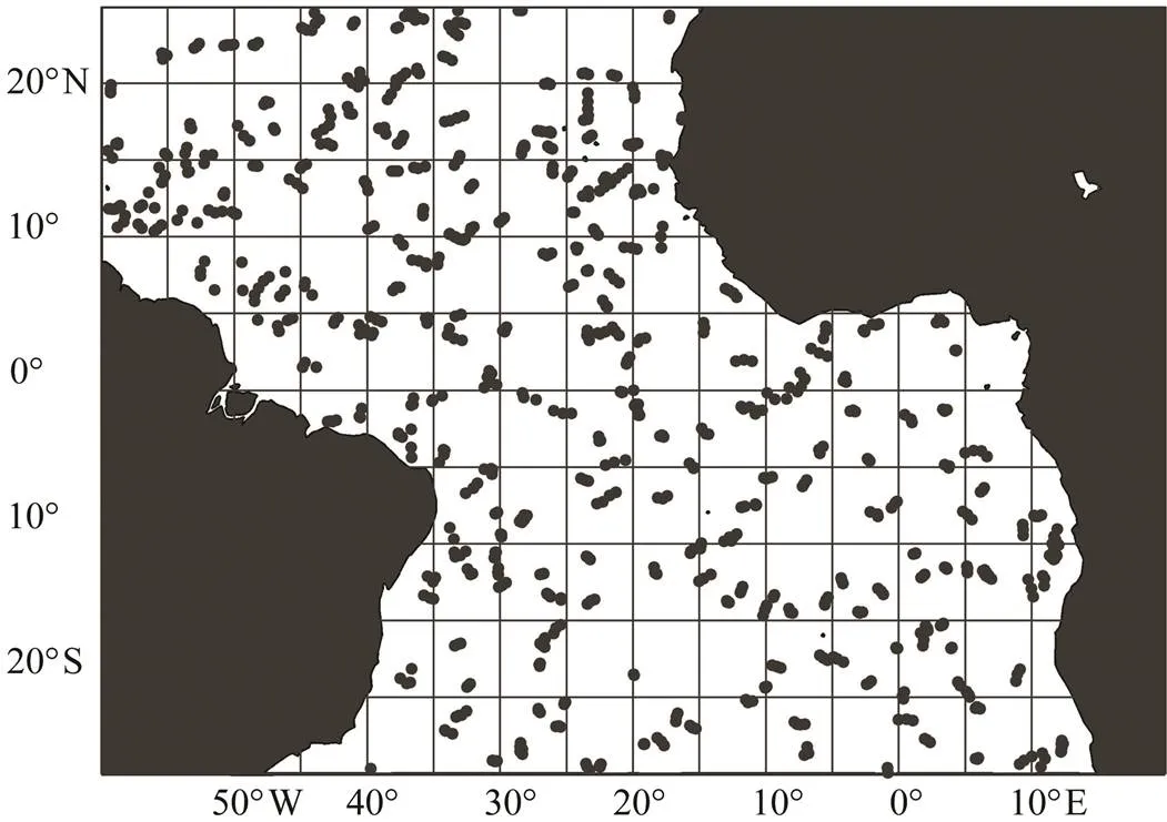
Fig.1 Study area and spatial distribution of Argo profile data in December 2016. The dot indicates the position of the Argo buoy.

Akima interpolation methods (Akima, 1970) were applied to fit the water temperature profile data into 2m in- tervals before calculating the thermocline and subsurface temperatures. Akima spline is a type of cubic spline that is relatively robust to outliers. Given a set of points (x,y), wherexstrictly increases, the Akima spline will go through each of the given points. At those points, its slopesis a function of the locations of the points (x−2,y−2) through (x+2,y+2). Specifically, we definemas the slope of the line segment from (x,y) to (x+1,y+1), namely, (y+1−y)/(x+1−x). Subsequently,sis defined as the following weight- ed average ofm−1andm:

The spline is defined as the piecewise cubic function whose value between xi and xi+1is the unique cubic polynomial p(x)that satisfies the four constraints: p(xi)=yi, p(xi+1)=yi+1, p´(xi)=si, and p´(xi+1)=si+1. Fig.2 shows a comparison of the scatter diagram and interpolation diagram.

We calculated the temperature gradient in the vertical direction using the following formula:

where Δand Δare the differences in temperature and depth.

2.3 Subsurface Environmental Factors

According to the method developed by Zhou. (2002), we used 0.05℃m−1as the threshold value to identify the thermocline (the upper and lower boundaries of temperature and depth)stepwise discriminant analysis. The de- tails of the computational and determination method can be found in Zhou. (2004) and Yang. (2012, 2013). If several thermocline layers were present at one site, then the upper and lower boundaries of temperature and depth were selected as those of the first and last thermocline layers, respectively.

The optimum temperature range (in the vertical direction, perpendicular to the sea surface) for bigeye tuna is 10–15℃ in the eastern Pacific Ocean (Hanamoto, 1987). The optimum temperature range for bigeye tuna in the Indian Ocean is 10–16℃, and hooking rates peak at 12– 13℃ (Mohir., 1997; 2001). In the central Atlantic Ocean, Song. (2004) reported that the optimum tem- perature range for bigeye tuna is 9–15℃, and the hooking rates peak at 12–13℃. Considering the above results, in this study, the temperature range of 9–15℃ was selected as the optimum temperature range of bigeye tuna in the Atlantic Ocean. The upper and lower limits of the optimum water temperature were 15℃ and 9℃, respectively, and their respective water depths (15 and9) were applied to identify the minimum and maximum swimming depths in the daytime. Their depth range was defined as the preferred swimming depth. The lower limit of the temperature (in the vertical direction, perpendicular to the sea surface) associated with the highest hooking rate (12℃) was defined as the preferred foraging depth (12) of bigeye tuna during the daytime in the Atlantic Ocean.

Weselected all the scattered depth values at 9℃, 12℃, and 15℃ and the temperature and depth values of theupper and lower boundaries of the thermocline in the hori- zontal direction for all years and months, grouped these values by months, and calculated the contour values at a 1˚×1˚ spatial resolution via Kriging interpolation methods (Yang., 2008). We also plotted the monthly distribution maps of the subsurface temperature and the ther- mocline (Yang., 2012, 2013, 2015). Given that the thermocline influences the vertical distribution of bigeye tuna (Bertrand., 2002; Abascal., 2018), the depth differences between the 12℃ isolines and the lower bound- ary of the thermocline (12) were calculated. To match the fishery data, all environmental data were averaged ac- cording to a 5˚×5˚ grid.

2.4 Data Analysis

By plotting12,9, and15 on a spatial overlay map with the monthly standardized, the potential foraging depth range, preferred swimming depth, and their influences on the longlineof bigeye tuna were cha- racterized.12 was used to analyze the relationship be- tween the average foraging depth and the thermocline.

We pooled the monthly data and calculated the first, second, and third quartiles (Q1–Q3). We selected the third quartile (Q3=5.06) as the threshold value. Standardizedvalues which greater than 5.06 were defined as ‘highs’. According to Andrade. (1999) and Zainud- din. (2008), we defined the regions with highvalues as hotspots (Zainuddin., 2008). The highdata were used to evaluate the spatial distribution of the fishing grounds, and the nominalwas standardized before analyzing the spatial distribution of the monthly.

According to their superiority as indicated by Shono (2014) and Li. (2015), support vector machines (SVMs) were selected as the standardization models. SVM is a pat- tern recognition method developed from statistical learn- ing theory based on the idea of structural risk minimize- tion principle (Sun and Zou, 2015). The assumption isthat there are training data sets ((x,y),=1, 2,∙∙∙,), wherexRandy.={1,2, ∙∙∙,x}is input data, and={1,2, ∙∙∙,y} is the output value of the model. The aim of SVR is to find an optimal hyper plane H. The distance of all the samples to H is small. We wish to predict a real- valued output() for the observed value. Thus, the regression function in high-dimensional feature space is(), whereis the weight vector, andis the threshold,:→is a transformation of the input space into a new space, which is usually a high dimension space. The penalty function is defined as

whereis an insensitive loss function. This problem is transformed into the optimal problemandby introducing relaxation variableand penalty factor:

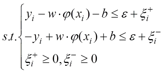
The input variables included year, month, latitude, and longitude; the nominalwas defined as the continu- ous response variable in the SVM model (Shono, 2014). MATLAB was used to create monthly standardizeddistribution maps and investigate the monthlydistribution patterns.

Using frequency analysis and the empirical cumulative distribution function (ECDF), we analyzed the relationshipbetween the oceanographic variables and highdur- ing the same period (Perry and Smith, 1994; Andrade., 1999; Zainuddin., 2008) and estimated the optimum ranges of variables.

Polynomial regression was used to develop an algori- thm for the vertical distribution of bigeye tuna (Hartokob, 2010; Sukresno., 2015):

whereis the probability of fishing zone formation (0– 100%), which indicates the potential value of the standardized;0,1, and2are the respective regression parameters; andis12 or12. The ECDF and polynomial regression were calculated using MATLAB.

To avoid overfit models, a GAM was used to examine the nature of the relationship between the nominaland the environmental and spatiotemporal variables. Following Maury. (2001), we assumed a normal distribution for log(+1). Considering that the lower depth boundary and temperature of the thermocline are important factors in the vertical and spatial distributions of bigeye tuna, these factors were included in the model. Finally, year, month, latitude, longitude, isothermal depth at 12℃ (12),12, and lower depth boundary of the thermocline () were selected as input variables. All explanatory variables were modeled as a spline function (=4). The GAM was constructed in the R programming environment using the GAM function in the mgcv package (Wood, 2006). Model selection was performed manually. We retained candidate predictors that were significant, minimized the Akaike information criteria (AIC), and increased the amount of explained deviance.

3 Results

3.1 Standardized CPUE

The mean absolute error of the SVM model was 1.15. The Spearman’s rank correlation of the nominal and stan- dardizedwas 0.86 (<0.001). The trends in the nominaland standardizedfor bigeye tuna in the tropical Atlantic are shown in Fig.3. The average standardizedwas lower than average nominaland oscillated slightly less than the latter. Overall, the re- lative abundance of bigeye tuna was unstable and low from 2007 to 2011, increased during 2011–2013, and de- creased from 2015 to 2017.

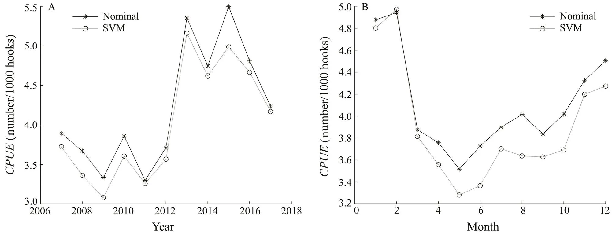
Fig.3 Yearly (A) and monthly (B) trends of nominal CPUE and CPUE standardized by support vector machine (SVM) for bigeye tuna from 2007 to 2017.

3.2 Potential Range of Preferred Swimming Depth

The preferred swimming depth of bigeye tuna in the tropical Atlantic was estimated based on9 and15 (Figs.4 and 5). The depth ranges were 100–450m for15 and 350–750 for9. The depth of the higher limit of the optimum water temperature (15℃) was approximately 150m, and the depth of the lower limit of the optimum water temperature (9℃) ranged from 350m to 400m around the equatorial region. Both depth contours showed a strong gradient north of 10˚N.9 and15 were 400–550m and 150–250m in the south, respectively, with an oblique pat- tern from South America 10˚S to Africa 25˚S. The depths in the equatorial zone and offshore of Namibia in the Atlantic were approximately 150 (Fig.5) and 350–400m (Fig.4), respectively.

Most of the standardizeds were observed at the depth range of 300–400m and 100–200m for9 and15 (Fig.6), respectively.

Most of the standardizeds were observed at the depth range of 300–400m and 100–200m for9 and15 (Fig.6), respectively.

3.3 Potential Preferred Foraging Depth and Effect on the CPUE Distribution

The average12 spatial distribution of bigeye tuna in the tropical Atlantic (Fig.7) showed that the topography of the estimated12 was similar each month, with a roughly striped zonal distribution for the annual mode. The preferred foraging depth was greater than 300m in the northern area, which started from 15˚N off West Africaand ended at 10˚N off South America. In the southern area, it started from 10˚S off South America and ended at 30˚S off West Africa. Between the two slopes, the preferred foraging depths ranged from 190m to 250m. The prefer- red foraging depth was between 250 and 270m from au- tumn to spring and lower than 250m during the summer in the Gulf of Guinea and adjacent waters. High standar- dizeds (>5.06) were observed in the areas where12 was mainly between 190 and 300m, whereas the stan- dardizedwas low when12 exceeded 300m. How- ever, there were scattered high standardizeds ob- served between the 15˚N and 20˚N zones, where the pre- ferred foraging depth was deeper than 300m, especially during December to February of the next year.

3.4 Vertical Distribution of Standardized CPUEs

The results of the ECDF are shown in Fig.8. The relationship between the standardizedand the two vari- ables reinforced the results obtained above. The cumula- tive distribution curves of the variables differed, and the degrees of the difference between the two curves (()) were highly significant (=0.05). The results showed a strong association between the standardizedand the two variables.12 was 168 to 322m (245m±77m, Fig.8A), and12 was 5 to 175m (90m±85m, Fig.8B). The frequency of standardizeds of bigeye tuna de- creased in areas outside of these favorable ranges.

Algorithms based on polynomial regression equations of bigeye tuna are presented in Fig.9. The results of vertical distribution analysis showed that bigeye tuna were found at approximately 12℃ (2=0.86) and below the lower boundary depth of the thermocline (2=0.80). Thus, the vertical distribution of standardizeds was high- lyaffected by the temperature of 12℃ and the thermocline.

The scatterplot of12 and the(Fig.10A) suggested that the standardizeds were observed in areas where12 ranged from 140m to 680m (mean=269m, s.d.=77m). Most of the standardizeds were con- centrated at 190–279m (71.5%, mode=220–240m). The standardizednumbers sharply decreased below 200m and above 300m.12 ranged from –120 to 529m, with 83.8% of the standardizeds distributed between –20 and 179m (mode=30–50m; Fig.10B). The standardizednumbers showed a sharply decreasing trend at sha- llow relative depths (<0m) but a gradual decline in the deeper depth range (>200m).

3.5 GAM Results

The results of GAM analysis indicated that seven predictor variables (year, month, latitude, longitude,12,12, and) were retained at the 5% level (Tables 1 and 2). The variable of month showed associatedvalues well above those found for the other variables. The GAMs ex- plained 27.8% of the null deviance. The general relationships between ln(1) and the seven variables were all nonlinear (Fig.11).

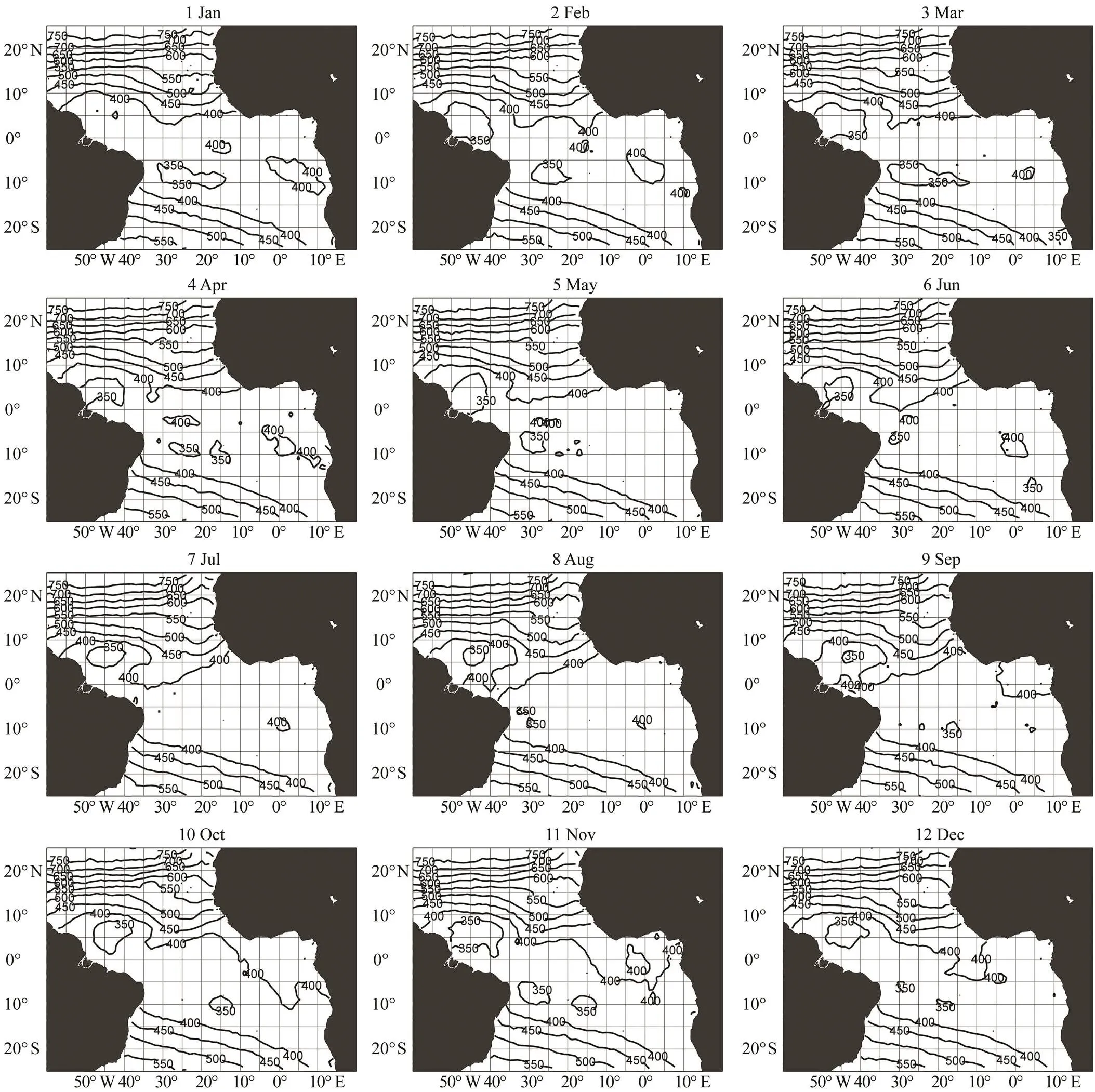
Fig.4 Monthly 9℃ contour (D9) map. Data aggregated and averaged from 2007 to 2017.

The effects of the seven variables on nominalwere nonlinear. Figs.11A and 11B show that the hooking rates were low before 2010 and then increased until 2015, decreased from January to May, and increased until October. The nominalvalues were at a low value at the south of 5˚N and quickly increasedat the north of 5˚N. The effect of latitude on the longline tuna fishing fleet was strong. Fig.11D indicates that thevalue was highest at approximately 40˚W, but the 95% confidence interval was relatively large. Most of the fishing effort of the longline tuna fishing fleet was concentrated near 30˚W.The effect of12 on theis shown in Fig.11E, where the curve continuously decreased with a negative effect. High hooking rates occurred between 200 and 300m in depth. Nominalvalues were low when the depth at 12℃ was deeper than 300m. The general relationship be- tween nominalandwas characterized by a convex shape (Fig.11F). The effect ofon theslowly increased from 50m and decreased from approximately 150m. Mosts were made withinlevels that ranged from 160 to 230m. The general relationship between nominaland12 was characterized by a concave shape (Fig.11G). Thedecreased as12 became deeper.

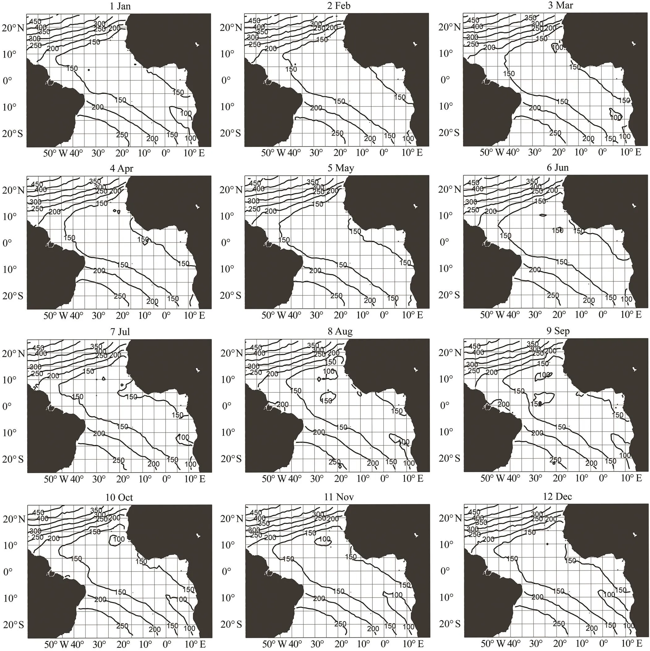
Fig.5 Monthly 15℃ contour (D15) map. Data aggregated and averaged from 2007 to 2017.

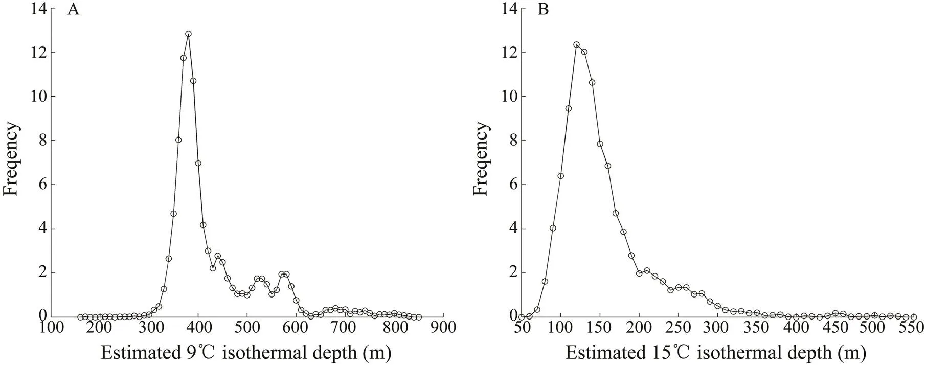
Fig.6 Relationships between D9 (A) and D15 (B) and standardized CPUEs from 2007 to 2017.

Fig.7 Monthly overlay map of the standardized CPUE and contour of the estimated 12℃ isothermal depths.

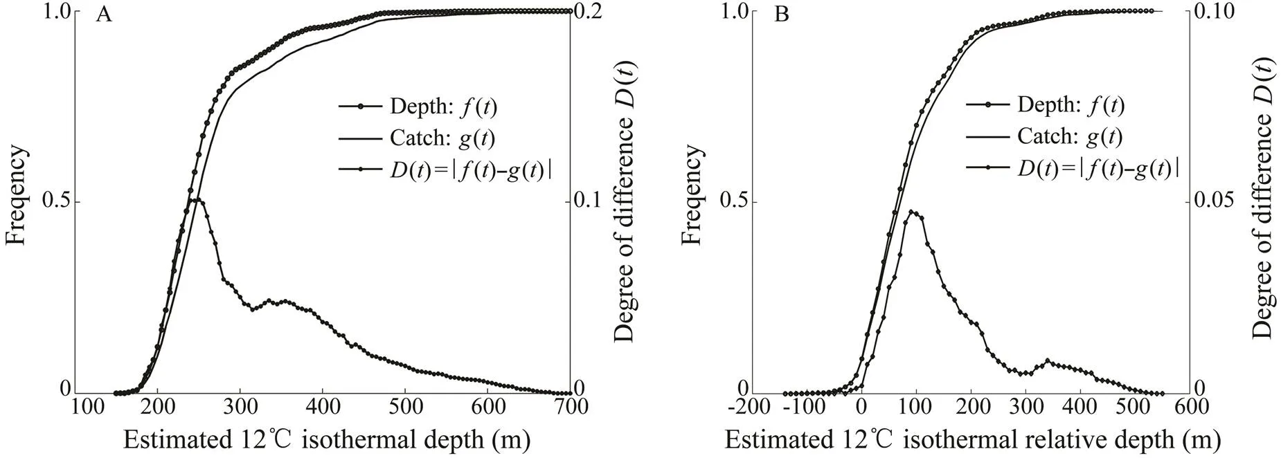
Fig.8 ECDF for D12(A) and RD12 (B) and frequency of CPUEs.

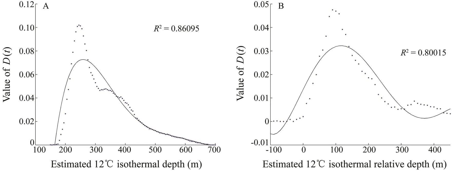
Fig.9 Vertical distribution analysis of bigeye tuna at D12 (A) and RD12(B).

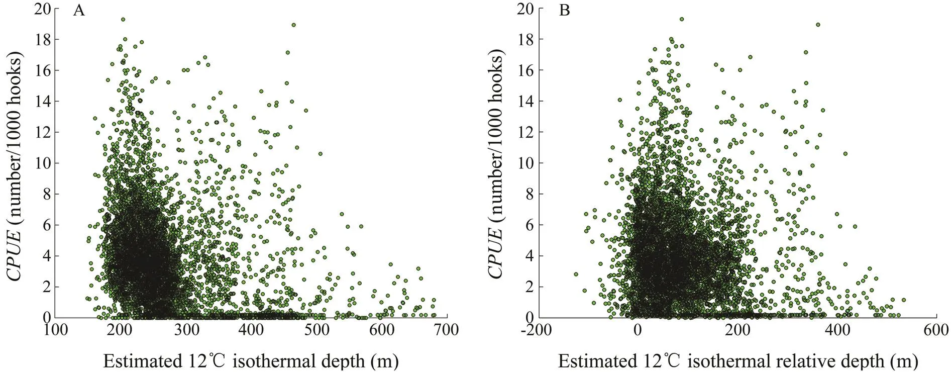
Fig.10 Scatterplots of D12(A) and RD12(B) and the standardized CPUE.

Table 1 Statistical characteristics of the model

Table 2 F-test for the significance of nonparametric effects

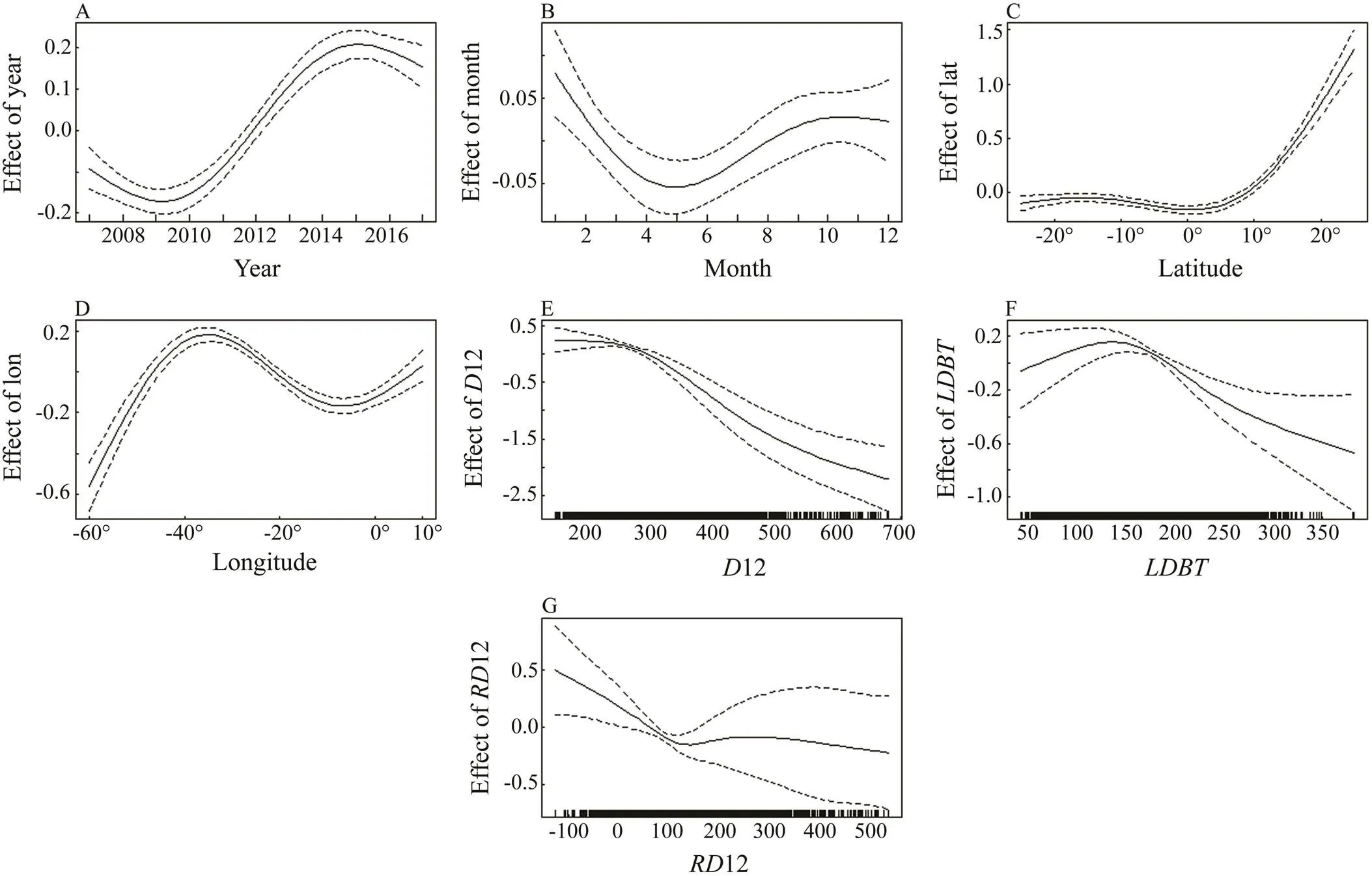
Fig.11 GAM-derived effects of six predictors on CPUE. A, year; B, month; C, longitude; D, latitude; E, D12; F, LDBT; G, RD12.

4 Discussion

4.1 Foraging Depth

The foraging layer of bigeye tuna in the tropical Atlantic was well below the thermocline. Vertical habitat quantification is important for estimating population trends fromtime series for pelagic species. The potential foraging depth range of bigeye tuna in the tropical Atlantic was evaluated with Argo data. On the basis of the depth ofcapture with longline fishing gear, the depth distribution ofAtlantic bigeye tuna ranged from 120 to 390m. Thewas the highest at 240–260.99m, followed by that at 270– 299.99m (Song., 2004). Yokawa. (2006) stated that the highestwas in the deepest layers (175–325m in absolute depth). In this study, the foraging depth of bigeye tuna in the tropical Atlantic was found from 100 to 400m and displayed spatial variation (Figs.4 and 5). The preferred foraging depth was mainly between 190 and 300m. The spatial distribution results of this research were con- sistent with those of previous studies (Song., 2004; Yokawa., 2006). Most of the highs were observed in an area where the average foraging depth was below the lower boundary of the thermocline, and the12 values were concentrated at 30–50m. Song. (2009) reported that most of the bigeye tunas are hooked below the thermocline. Bigeye tuna can forage in deep coldwater because they have evolved unique physiological and mor- phological adaptations such as vascular countercurrent heat exchangers. Together with behavioral strategies, this allows them to maintain their body temperature below the ther- mocline for a long period and exploit food resources more effectively than other fishes (Brill., 2005).

4.2 Effects on Hooking Rates

Highs were concentrated in the central Atlantic and offshore of South America, and scattered in the central Atlantic and offshore of Africa. Seasonal fishing grounds were noted off the coast of Angola and Namibiaand in the open ocean (Fig.7). Data collection month had a statis-tically significant influence on. The trends ofsuggested that the catch rates after 2012 were higher than those before 2012. The data were not separated into two periods because these data were deep longline data; this trend reflected the situation of fish stock. Seasonal and spa- tial distribution patterns of fishery data were observed for bigeye tuna (Lam., 2014; Lan., 2018). The vari- ation inis the natural characteristic of fishery. Theseresults were in accordance with the standardized index cal- culated in the report of the 2018 ICCAT bigeye tuna stock assessment meeting (ICCAT, 2018).

The vertical structure of the water column influences the vertical distribution of bigeye tuna and the efficiency of longline gear, and further affects the spatial distribution of commercial. Most of the high hooking rates were observed in the shallow depth (190–300m) for12, which ranged from 190 to 700m (Fig.10). Prince and Goodyear (2006) stated that a suitable depth distribution is impor- tant to the ecology of pelagic fishes. The distinct diurnal shift in the diving behavior of bigeye tuna suggests that bigeye tuna may generally inhabit at deeper ocean. They are less aggregated when the vertical depth distribution or ther-mocline deepens because of their extensive vertical migra- tions. In this area, this phenomenon reduced their vulner- ability to shallow longline fishing gear (Lan., 2018). Bertrand. (2002) stated that the deep foraging depth can reduce the vulnerability of bigeye tuna to longline gear.Thus, the hooking rate and the number ofs were low in the area to the north of the slope that starts from 15˚N in West Africa and ends at 10˚N in South America, where12 is deeper than 400m (Fig.7). However, the hooking rate was low in the area where12 andbecame shallow (Fig.11). The efficiency of longline gear differs de- pending on the depth of the hooks and the swimming depth of the fish (Matsumoto., 2004). This phenome- non may occur because most of the longline hook depths are deeper than the thermocline.

4.3 Improvement to CPUE Estimation

Longline catchability also depends on the vertical distri- bution of bigeye tuna and should be considered instandardization. According to Hinton and Nakano (1996), the determinant for blue marlin () is the difference of temperature between the surface layer and waters below the thermocline rather than the specific water temperature. In this study, the spatial model and GAM results indicatd that the hooking rates were affected by the thermocline and average foraging depth. These effects may not be independent. Warm water preferences are well known for tuna species. Bigeye tunas preferentially stay in zones where the sea surface temperature (SST) is higher than 26℃ (Zhu and Xu, 2008). However, high hooking rates were observed offshore of Namibia, where the up- per temperature of the thermocline was lower than 20℃ (Fig.11) (Yang., 2013). Conversely, small individuals of bigeye tuna were caught in the north of the slope from 15˚N of West Africa to 10˚N of South America, where the upper temperature of the thermocline was higher than 26℃ (Yang., 2013). The above difference suggested that the catchability of bigeye tunalongline was also in- fluenced by the thermocline and average foraging depth.

4.4 Outlook

The fishery data did not contain information on the num- ber of hooks between floats (NHBF). The NHBF repre-sents the depths of the hooks and is considered to indicate the targeted species. We assumed that there is not sub- stantial annual difference in theof bigeye tuna. The monthly bigeye tunawas used for the analysis, and the results of this analysis might contain bias. In future research, we will present the effects of the NHBF by us- ing the fine-scale dataset and the annual variation in.

5 Conclusions

In this study, we used Argo profile data to investigate the potential vertical distribution of bigeye tuna and determine whether the potential vertical distribution influences the spatial distribution of longlines. The pre- ferred swimming depth of bigeye tuna in the tropical Atlantic is from 100 to 400m and displays spatial variation. The preferred foraging depth is mainly between 190 and 300m and below the thermocline. The swimming depth and foraging depth are influenced by water temperature, which further affects the hooking rates of the longline. Most of the standardizeds are observed at the preferred foraging depths, which are shallower than 300m, and peak at 30–50m12. GAM analysis indicates that the general relationship between the nominalandis characterized by a dome shape with a peak at ap- proximately 190m. Our results provide new insights into how oceanographic features influence the habitat of tro- pical pelagic fish and fisheries and how fisheries exploit these fish using a new tool (Argo profile data). Fortunately, most of the variables that may influence fish are present in the Argo data. In the future, Argo buoy data could be an important tool to describe the habitat of oceanic fish, not only that of bigeye tuna.

Acknowledgements

This study was supported by the National Natural Science Foundation of China (No. 41606138), the Special Funds of Basic Research of Central Public Welfare Institute (Nos. 2019T09, 2016Z01-02), the National Key Research and Development Project of China (No. 2019YFD 0901405), and the Fund of Key Laboratory of Open-Sea Fishery Development, Ministry of Agriculture, P. R. Chi- na (No. LOF2018-01).

Abascal, F. J., Peatman, T., Leroy, B., Nicol, S., Schaefer, K., Fuller, D. W., and Hampton, J., 2018. Spatiotemporal variability in bigeye vertical distribution in the Pacific Ocean., 204: 371-379.

Akima,H., 1970. A newmethod of interpolation and smooth curve fitting based on local procedures., l7 (4): 589-602.

Andrade, H. A., and Garcia, A. E., 1999. Skipjack tuna in relationto sea surface temperature off the southern Braziliancoast.,8(4): 245-254.

Arrizabalaga, H., Pereira, J. G., Royer, F., Galuardi, G., Goni, N., Artetxe, I., Arregi, I., and Lutcavage, M., 2008. Bigeye tuna () vertical movements in the Azores Islands determined with pop-up satellite archival tags., 17 (2): 74-83.

Bertrand, A., Josse, E., Bach, P., Gros, P., and Dagorn, L., 2002. Hydrological and trophic characteristics of tuna habitat: Consequences on tuna distribution and longline catchability., 59 (6): 1002- 1013.

Bigelow, K. A., and Maunder, M. N., 2007. Does habitat or depth influence catch rates of pelagic species?, 64 (11): 1581-1594.

Brill, R. W., Bigelow, K. A., Musyl, M. K., and Fritsches, K. A., 2005. Bigeye tuna () behavior and physiology and their relevence to stock assessments andfishery biology., 57 (2): 142-161.

Brill, R. W., Block, B. A.,Boggs, C. H., Bigelow, K. A., Freund, E. V., and Marcinek, D. J., 1999. Horizontal movements and depth distribution of large adult yellowfin tuna() near the Hawaiian Islands, recorded using ultrasonic telemetry: Implications for the physiological ecology of pelagic fishes.,133(3):395-408.

Dagorn, L., Bach, P., and Josse, E.,2000. Movement patterns of large bigeye tuna () in the open ocean, determined usingultrasonic telemetry., 136 (2): 361- 371.

Deary, A. L., Moret-Ferguson, S., Engels, M., Engels, M., Zettler, E., Jaroslow, G., and Sancho, G., 2015. Influence of central Pacific oceanographic conditions on the potential vertical habitat of four tropical tuna species., 69 (4): 461-475.

Evans, K., Langley, A., Clear, N. P., Williams, P., Patterson, T., Sibert, J.,Hampton, J., and Gunn, J. S., 2008. Behaviour and habitat preferences of bigeye tuna () and their influence on longline fishery catches in the western Coral Sea., 65(11): 2427-2443.

Fuller, D. W., Schaefer, K. M., Hampton, J., Caillot, S., Leroy, B., and Itano, D., 2015. Vertical movements, behavior, and habi- tat of bigeye tuna () in the equatorial central Pacific Ocean.,172: 57-70.

Furukawa, S., Tsuda, Y., Nishihara, G. N., Fujioka, K., Ohshimo, S., Tomoe, S., Nakatsuka, N., Kimura, H., Aoshima, T., Kane-hara, H., Kitagawa, T., Chiang, W. C., Nakata, H., and Kawabe, R., 2014. Vertical movements of Pacific bluefin tuna () and dolphinfish () relative to the thermocline in the northern East China Sea.,149: 86-91.

Hanamoto, E., 1987. Effect of oceanographic environment on bigeye tunadistributions., 51 : 201-216.

Hartokob, A., 2010. Spatial distribution ofsp, vertical and horizontal sub-surface multilayer temperature profiles ofArgo float data in Indian Ocean., 14 (1): 61-74.

Hinton, M. G., and Nakano, H., 1996. Standardizing catch and effort statistics using physiological, ecological, or behavioural constraints and environmental data, with an application to blue marlin () catch and effort data from the Ja- panese longline fisheries in the Pacific.,21: 169-200.

Holland, K. N., and Sibert, J. R., 1994. Physiological thermoregulation in bigeye tuna,, 40 (3): 319-327.

Houssard, P., Lorrain, A., Tremblay-Boyer, L., Allain, V., Graham, B. S., Menkes, C. E., Pethybridge, H., Couturier, L. I. E., Point, D., and Leroy, B., 2017. Trophic position increases with thermocline depth in yellowfin and bigeye tuna across the western and central Pacific Ocean., 154: 49-63.

Howerll, E. A., Hawn, D. R., and Polovina, J. J., 2010. Spatiotemporal variability in bigeye tuna () dive be- havior in the central North Pacific Ocean., 86 (1-2): 81-93.

ICCAT Tropical Tuna Working Group, 2018. Report of the 2018 ICCAT bigeye tuna stock assessment meeting. Bet Stock Assessment Meeting, Pasaia, Spain.

Josse, E., Bach, P., and Dagorn, L., 1998. Simultaneous obser- vations of tuna movementsand their prey by sonic tracking and acoustic surveys., 371-372 (1): 61-69.

Lam, C. H., Galuardi, B., and Lutcavage, M. E., 2014. Move- ments and oceanographic associations of bigeye tuna () in the Northwest Atlantic., 71 (10): 1529-1543.

Lan, K. W., Lee, M. A., Chou, C. P., and Vayghan, A. H., 2018. As- sociation between the interannual variation in the oceanic environment and catch rates of bigeye tuna () in the Atlantic Ocean.,27 (5): 396-407.

Laurs, R. M., Fiedler, P. C., and Montgomery, D. R., 1984. Al- bacoretuna catch distributions relative to environmental featuresobserved from satellites.,31 (9): 1085-1099.

Lee, P. F., Chen, I. C., and Tzeng, W. N., 2005. Spatial and temporal distribution patterns of bigeye tuna () in the Indian Ocean., 44 (2):260-270.

Matsumoto, T., Kitagawa, T., and Kimura, S., 2013a. Vertical be- havior of bigeye tuna () in the northwestern Pacific Ocean based on archival tag data., 22 (3): 234-246.

Matsumoto, T., Kitagawa, T., and Kimura, S., 2013b. Considerations on diving patterns of bigeye tunabased o archival tag data., 79 (1): 39-46.

Matsumoto, T., Saito, H., and Miyabe, N., 2004. Swimming behavior of adult bigeye tuna using pop-up tags in the central Atlantic Ocean., 57 (1): 151-170.

Maury, O., Gascuel, D., Marsac, F., Fonteneau, A., and Rosa, A. D., 2001. Hierarchical interpretation of nonlinear relationships linking yellowfin tuna () distribution to the environment in the Atlantic.,58(3):458-469.

Mohri, M., and Nishida, T., 1999. Distribution of bigeye tuna () and its relationship to the environmental conditions in the Indian Ocean based on the Japanese longline fisheries information., 2: 221-230.

Mohri, M., and Yasuaki, T., 1997. Vertical distribution and opti- mum temperature of bigeye tuna () in the east- ern tropical Indian Ocean based on regular and deep tuna longline catches.,46: 13-20 (in Japanese).

Musyl, M. K., Brill, R. W., Boggs, C., Curran, D. S., and Kazama,T. K., 2003. Verticalmovements of bigeye tuna () associated with islands, buoys,and seamounts near the main Hawaiian Islands from archival tagging data., 12 (3): 152-169.

Perry, R. I., and Smith, S. J., 1994. Identifying habitat associations of the marine fishes using survey data: An application to the northwest Atlantic., 51 (3): 589-602.

Prince, E. D., and Goodyear, C. P., 2006. Hypoxia-based habitat compression of tropical pelagic fishes., 15 (6): 451-464.

Schaefer, K. M., and Fuller, D. W., 2010. Vertical movements, be- havior, and habitat of bigeye tuna () in the equatorial eastern Pacific Ocean,ascertained from archival tag data.,157 (12): 2625-2642.

Shono, H., 2014. Application of support vector regression to CPUE analysis for southern bluefin tunaand its comparison with conventional methods., 80 (5): 879-886.

Song, L. M., Xu, L. X., and Chen, X. J.,2004. Relationship be- tween bigeye tuna vertical distribution and the temperature, salinity in the central Atlantic Ocean., 11 (6): 561-566 (in Chinese with English abstract).

Song, L. M., Zhou, J., Zhou, Y. Q., Nishida, T., Jiang, W. X., and Wang, J. Q., 2009. Environmental preferences of bigeye tuna,, in the Indian Ocean: An application to a long-line fishery., 85 (2): 153-171.

Sukresno, B., Hartoko, A., and Sulistyoc, B., 2015. Empirical cu- mulative distribution function (ECDF) analysis ofsp. using Argo float sub-surface multilayer temperature data in Indian Ocean south of Java., 23: 358-367.

Sukresno, B., Murdimanto, A., Hanintyo, R., Jatisworo, D., and Ku- suma, D. W., 2019. The use of CMEMS and Argo float data for bigeye tuna fishing ground prediction., 246 (1): 1-15.

Sun, X. Q., and Zou, L. Y., 2015. Research on application of su- pport vector machine in fault recognition of bearings.,36 (2):12-15.

Takano, A., Yamazaki, H., and Nagai, T., 2009. A method to esti- mate three-dimensional thermal structure from satellite altimetry data.,26(12): 2655-2664.

Ward, P., and Myers, R. A., 2005. Inferring the depth distribution of catchability for pelagic fishes and correcting for variations in the depth of longline fishing gear., 62 (5): 1130-1142.

Wood, S. N., 2006.. CRC Press, Boca Raton, FL, 217-255.

Yang, S. L., Ma, J. J., and Wu, Y. M., 2015. Relationship be- tween temporal-spatial distribution of fishing grounds of big- eye tuna () and thermocline characteristics in the Atlantic Ocean., 35 (3): 1-9.

Yang, S. L., Ma, J. J., Wu, Y.M., and Zhou, W.F.,2008. Study on the reconstruction of Pacific temperature arena withArgo data based on the Kriging methods.,30(1): 13-18 (in Chinese with English abstract).

Yang, S. L., Ma, J. J., Wu, Y. M., Tang, F. H., Zhang, H., and Zhou, S. F.,2012. Seasonal variability of temperature profile inandfishing ground in the Indian Ocean., 36 (7): 97-103 (in Chinese with English abstract).

Yang, S.L., Zhang, S.M., Jiang, X.W., Zou, B., Hua, C. J., and Zhou, W. F., 2013. Seasonal variability of thermocline inandfishing ground in the tro- pic Atlantic Ocean., 32(3): 349-357 (in Chinese with English abstract).

Yokawa, K., Saito, H., Kanaiwa, M., and Takeuchi, Y., 2006. Ver- tical distribution pattern of CPUE of Atlantic billfishes and associated species estimated using longline research data.,79(3): 623-634.

Zainuddin, M., Saitoh, K., and Saitoh, S., 2008. Albacore () fishing ground in relation to oceanographic con- ditions in the western North Pacific Ocean using remotely sensed satellite data.,17(2): 61-73.

Zhou, Y. X., Li, B. L., Zhang, Y. J., and Ba, L. C.,2002. World oceanic thermocline characteristics in winter and summer.,21 (1): 16-22 (in Chinese with English abstract).

Zhu, G.P., and Xu, L.X., 2008. Hooking rates distribution ofin tuna longliningground and its relationship with SST in thewestern tropical Atlantic Ocean.,30(1): 8-12 (in Chinese with English abstract).

. Tel: 0086-21-61900311

E-mail: lmsong@shou.edu.cn

June 20, 2019;

August 4, 2019;

December 24, 2019

(Edited by Qiu Yantao)