Diffusion Characteristics of Swells in the North Indian Ocean

ZHENG Chongwei,LIANG Bingchen, CHEN Xuan, WU Guoxiang,SUN Xiaofang, and YAO Jinglong

Diffusion Characteristics of Swells in the North Indian Ocean

ZHENG Chongwei1), 2), 3), #, *,LIANG Bingchen4), #, CHEN Xuan5), WU Guoxiang4),SUN Xiaofang1), and YAO Jinglong6)

1) Dalian Naval Academy, Dalian 116018, China 2) State Key Laboratory of Numerical Modeling for Atmospheric Sciences and Geophysical Fluid Dynamics (LASG), Institute of Atmospheric Physics, Chinese Academy of Sciences, Beijing 100029, China 3) Shandong Provincial Key Laboratory of Ocean Engineering, Ocean University of China, Qingdao 266100, China 4) College of Engineering, Ocean University of China, Qingdao 266100, China 5) The 75839 Army, People’s Liberation Army, Guangzhou 510510, China 6) South China Sea Institute of Oceanology, Chinese Academy of Sciences, Guangzhou 510301, China

Research on the diffusion characteristics of swells contributes positively to wave energy forecasting, swell monitoring, and early warning. In this work, the South Indian Ocean westerly index (SIWI) and Indian Ocean swell diffusion effect index (IOSDEI) are defined on the basis of the 45-year (September 1957–August 2002) ERA-40 wave reanalysis data from the European Centre for Medium-Range Weather Forecasts (ECMWF) to analyze the impact of the South Indian Ocean westerlies on the propagation of swell acreage. The following results were obtained: 1) The South Indian Ocean swell mainly propagates from southwest to northeast. The swell also spreads to the Arabian Sea upon reaching low-latitude waters. The 2.0-meter contour of the swell can reach northward to Sri Lankan waters. 2) The size of the IOSDEI is determined by the SIWI strength. The IOSDEI requires approximately 2–3.5 days to fully respond to the SIWI. The correlations between SIWI and IOSDEI show obvious seasonal differences, with the highest correlations found in December–January–February (DJF) and the lowest correlations observed in June–July–August (JJA). 3) The SIWI and IOSDEI have a common period of approximately 1 week in JJA and DJF. The SIWI leads by approximately 2–3 days in this common period.

Indian Ocean; swell; Indian Ocean swell diffusion effect index

1 Introduction

The North Indian Ocean, one of the two major water bodies of the Maritime Silk Road, includes some of the world’s most important waterways, and its natural environment is complex and extensively affected by the swell of the ocean. Swells have astounding destructive force and can cause a ship to experience sagging, hogging, and, eventually, serious damage. Several studies have found that swells play a dominant role in mixed waves (Ardhuin, 2009; Dong, 2009; Liang, 2016; Yan, 2020). Because swells have high energy and good stability (Zheng, 2018), swell power generation has recently become an important development direction for marine green energy. Studies have also shown that swells can travel long distances with little energy loss (Munk, 1963), which means understanding the characteristics of these waves can be useful for monitoring them and improving the precision of wave forecasting. The ocean is an important regulator of global climate change, and wavesare one of the most active elements of the sea–air interface. Therefore, an in-depth study on swell characteristics has practical value for wave energy development, swell monitoring, early warning, navigation route planning, air-sea interaction analysis, and global climate change research.

Chen(2002)found several swell pools in the tropical East Pacific, tropical East Atlantic, and tropical East Indian Oceans. Zheng(2013) found two other swell pools in the tropical western Pacific and mid-western tropical Indian Oceans by using ERA-40 wave reanalysis data from the European Centre for Medium-Range Weather Forecasting (ECMWF). Also using ERA-40 wave reanalysis data, Semedo (2010) found that Atlantic swells clearly propagate from north to south during winter in the Northern Hemisphere. Liu and Yu (1998) analyzed the wave characteristics of the North Indian Ocean on the basis of meteorological ship reports for the period 1980–1990. These studies have found that the wind-sea wave and swell wave directions agree well during the monsoon season. The southwest wind speed is faster than the northeast wind speed. Zhang(2003) analyzed the wave characteristics of the South Indian Ocean by using a 45-year meteorological ship report and found that the variation of the wave field in the North Indian Ocean is more obvious than that in the South Indian Ocean. The region north of 10˚S is the monsoon area, while other sea regions are areas wherein southeastward waves prevail in the trade winds. The region south of 40˚S typically has waves directed from the west. Mei(2010) analyzed the wave and wind fields of the South China Sea and North Indian Ocean based on hindcast wave data and pointed out that areas with large wave heights in the east-central equatorial Indian Ocean may be caused by swells generated by the South Indian Ocean westerly belt. Using ERA-40 wave reanalysis data, Zheng(2016) analyzed the temporal and spatial distributions of wind-sea, swell, and mixed waves in the Indian Ocean. The team showed that swells play a dominant role in the characteristics of mixed waves from January to May and from September to December while wind-sea waves play a dominant role from June to August in the Arabian Sea. In addition, swells heavily influence the characteristics of mixed waves in the Bay of Bengal throughout the year. The strength of the west wind in the southern Indian Ocean determines the stretch of swells toward northern waters. Alevs (2006) found that swells of the South Indian Ocean westerly belt can usually propagate toward the tropical and subtropical waters of the Indian and Pacific Oceans.

A good understanding of wind-sea and swell separation technology, swell index, and swell pools has been achieved through the combined contributions of previous researchers. However, overall, research on swell propagation is stillrelatively rare. In the present work, the impact of the SouthIndian Ocean westerlies on the propagation of swell acreage is analyzed by using ERA-40 wave reanalysis data.

2 Methodology and Data

2.1 Data

ERA-40 wave reanalysis data from the ECMWF are used in this work. The data have a spatial range of 90˚S–90˚N, 180˚W–180˚E, and the time series is from September 1957 to August 2002. The spatial resolution is 1.5˚×1.5˚, and the temporal resolution is 6h. From December 1991 to May 1993, the errors are slightly larger due to an external processing error. The significant wave height from the ERA-40 wave reanalysis data is overestimated at low wave heights and underestimated at high wave heights (Sterl and Caires, 2005; Caires and Sterl, 2005; Zheng, 2018). Semedo(2011)analyzed the seasonal characteristics and long-term trends of wind-sea, swell, and mixed waves using ERA-40 wave reanalysis data. Sterl and Caires (2005) also used these data to analyze the wave climate of global oceans. The most important issue in these data involves the separation of wind seas and swells. Previous researchers made great contributions to the separation of wind seas and swells (Samiksha, 2012). However, separating wind seas from swells in a wide range of sea areas remains difficult because of the lack of many wave spectrum observations. Compared with other wave reanalysis datasets with separation of wind seas and swells, the ERA-40 wave reanalysis dataset processes the longest time series until now (Zheng, 2013). Therefore, the ERA-40 wave reanalysis dataset is currently the best choice for analyzing swell characteristics.

2.2 Methodology

The author defines the South Indian Ocean westerly index (SIWI) on the annual and monthly scales. The intensity of the South Indian Ocean westerlies is closely related to the northward propagation of swells. This study defines the SIWI and Indian Ocean swell diffusion effect index (IOSDEI) with a high time resolution (, 6h) to accurately analyze the influence of the South Indian Ocean westerlies on swell propagation in the Indian Ocean with time. The SIWI and IOSDEI are used to analyze the impact of the South Indian Ocean westerlies on the propagation of swell acreage quantitatively.

SIWI: Previous studies showed that the sea surface wind speed and swell wave height of the South Indian Ocean roaring westerly wind belt (40˚–60˚S, 30˚–120˚E) are much higher than those of other sea areas and that the swell in this area propagates northward. Therefore, the present study selects this area to investigate the impact of sea surface wind speed on the swell in the area and explore the characteristics of the northward propagation of large swells. The 10-meter sea surface wind speed of the South Indian Ocean westerly over this area at 00:00 on January 1, 1958 is regionally averaged, and the regional average wind speed at this time, which is regarded as the SIWI at this moment, is obtained. Using the same method, the 6-hourly SIWIs for the next 45 years (September 1957–August 2002) are obtained.

IOSDEI: Zheng (2018) found that the 2.0-meter contour of swell wave height can emphasize the northward propagation and southward contraction characteristics of swells in the Indian Ocean very well. Thus, the area covered by the 2.0-meter swell contour under the influence of the Indian Ocean westerly zone is selected as an index in this work to describe the strength of swells generated by the South Indian Ocean westerlies. The area within continuous 2-meter isolines is counted to avoid the influence of swells generated by the monsoon. Unfortunately, this process cannot completely exclude the swells generated by monsoons. In future work, designing an algorithm to determine the swells generated by monsoons accurately may be necessary. For example, the area covered by the 2.0-meter swell contour under the influence of the South Indian Ocean westerly zone at 00:00 on January 1, 1958 is regarded as the IOSDEI at this moment. Using the same method, the 6-hourly IOSDEIs for the next 45 years are obtained.

3 Strength of the South Indian Ocean Westerlies and Swell Diffusion

3.1 Phenomenon of Swell Propagation

Research shows that the 2.0-meter contour of swell wave heights in the South Indian Ocean demonstrates obvious characteristics of northward extension and southward contraction on a monthly scale. The present study focuses on the swell propagation in the South Indian Ocean on a weekly scale. A strong swell process generated by the roaring westerlies in the South Indian Ocean (June 2, 1979 00:00–June 13, 1979 18:00), hereinafter referred to as a ‘westerly strong swell’, is randomly selected to exhibit the spatial distribution of the strong swell field, as shown in Fig.1 (left). The sea surface wind field during this period is also presented in Fig.1 (right) to confirm that the swell is generated in the westerly zone, rather than another area, and propagates northward. Here, for easy observation, the unit vector arrow represents the swell direction, and the background color represents the swell wave height (H).

On February 2, 1979, the swells of the South Indian Ocean westerly are relatively weak.His basically within 3.5m, and the range ofHgreater than 4.0m is small. On February 3,Hincreases along with the strength of the South Indian Ocean westerlies. The range ofHabove 4.0m is significantly larger than that on the previous day, and an area ofHgreater than 4.5m could be observed. On February 4, the intensity of the swells further increases during eastward propagation; a swell area of 5.0m or greater is noted. On February 5, the strength of the large-value center of swells decreases. However, the range ofHgreater than 3.5m reaches its peak. After February 6, the swell center continues to move eastward and weaken. The 2.0-meter swell contour is mainly transmitted to the northeast, and the coverage continues to expand. During the propagation of swells, the 2.0-meter contour can extend northward to the waters near Sri Lanka.

Overall, the strong swells generated by the westerlies strengthen from February 2 to February 5 and gradually weaken from February 6 to February 9. The strong swell generated by the westerlies gradually spreads from southwest to northeast over time. At the same time, the range of swells above 2.0m in the mid-low latitudes of the South Indian Ocean gradually narrows toward the southeast. The strong swell generated by the westerlies shows apparent quasi-weekly oscillation when the intensity ofHis greater than 2.0m. The daily swell wave fields in January, April, July, and October of 1979, 1990, 1995, and 2000 are drawn to prove that this observation is not an accidental phenomenon. The propagation phenomenon is noticeably widespread in the strong swells generated by the westerlies. The intensity of strong swells generated by the westerlies and the area range of swells under the influence of the Indian Ocean westerlies demonstrate quasi-weekly oscillation phenomena similar to those of the south- west monsoon, and the cold air has periodicity. Seasonal variations in the intensity of strong swells generated by the westerlies and the northward propagation extent of these swells are not obvious. Zhang(2003)pointed out that the Indian Ocean north of 10˚S is the monsoon climate zone, that other sea areas are the trade wind zone wherein southeast waves prevail throughout the year, and that westward waves prevail south of 40˚S; the results of the present study are consistent with these findings.

Alves (2006) pointed out that the swells generated by the South Indian Ocean westerlies are usually spread east- ward to the tropical and subtropical regions of the Indian Ocean and the Pacific Ocean. The results of the present study are basically consistent with those of Alves, although the main propagation direction of the strong swells generated by the westerlies is from southwest to northeast and the swells can reach low latitudes in this work. The swells also extend to the Arabian Sea. The impact of swells generated by the South Indian Ocean westerlies on the Arabian Sea is far less significant than that on the Bay of Bengal, which is consistent with the results of Samiksha(2012). The direction of the swells of the Indian Ocean generally spreads northward in an anti-C shape. Because of the Coriolis force effect, the swells produced by the South Indian Ocean westerlies are gradually deflected northward during northeastward propagation. When the swells generated by the westerlies spread to the central Indian Ocean, they tend to spread to the northwest, which results in the emergence of anti-C-type features throughout the Indian Ocean. Furthermore, the overall topography of the Indian Ocean reveals that the mid-ocean ridge is distributed in the middle of the Indian Ocean, shows a herringbone shape, and penetrates the North Indian Ocean. Whether the terrain affects the propagation path of swells requires further research.

3.2 Seasonal Periods of the Westerly Strength and the Range of Swell Diffusion

Fig.1 reflects the existence of quasi-weekly oscillation phenomena in the SIWI and IOSDEI. The results of wavelet analysis that quantitatively calculates the intraseasonal periods of the SIWI and IOSDEI are shown in Fig.2. In June-July-August (JJA, Figs.2a, 2b), the SIWI has a 4–8-day cycle that is especially obvious in July. The IOSDEI lasts for a period of 7.5–16 days from June to July and a period of 4–8 days in August. In December–January–February (DJF, Figs.2c, 2d), the SIWI has a 4–8-day cycle in early to mid-December, no significant cycle in late December and early to mid-January, and a significant 4–8-day period in late January and February. The IOSDEI has a significant 8-day period in early December and January, as well as periods lasting over 8 days in late January and February. Overall, the IOSDEI has a significant 8-day period in JJA and DJF, indicating quasi-weekly oscillation. The SIWI also shows quasi-weekly oscillation, but it is not as obvious as that of the IOSDEI.

To rule out the contingency of a quasi-weekly oscillation in the IOSDEI, we count every 6-hour IOSDEI for the Indian Ocean in JJA and DJF in 1990, 1995, and 2000 and then calculate the period of the IOSDEI using wavelet analysis. Because of space limitations, only the results of 1990 and 1995 are listed in Fig.3. The IOSDEI shows very significant 8-day periods (, quasi-weekly oscillation) in JJA and DJF in 1990 and 1995.

Studies have pointed out that roaring westerlies show frequent cyclonic activity with an average of one cyclone passing every 2–3 days. The results of this paper reveal that the SIWI and IOSDEI have quasi-weekly oscillations. In future work, analyzing the relationship between westerly cyclones and strong swells generated by the westerlies may be necessary to understand the excitation mechanism and propagation characteristics of strong swells generated by the westerlies. The results of such analyses could provide a reference for the construction of the Maritime Silk Road and Antarctic development and utilization.

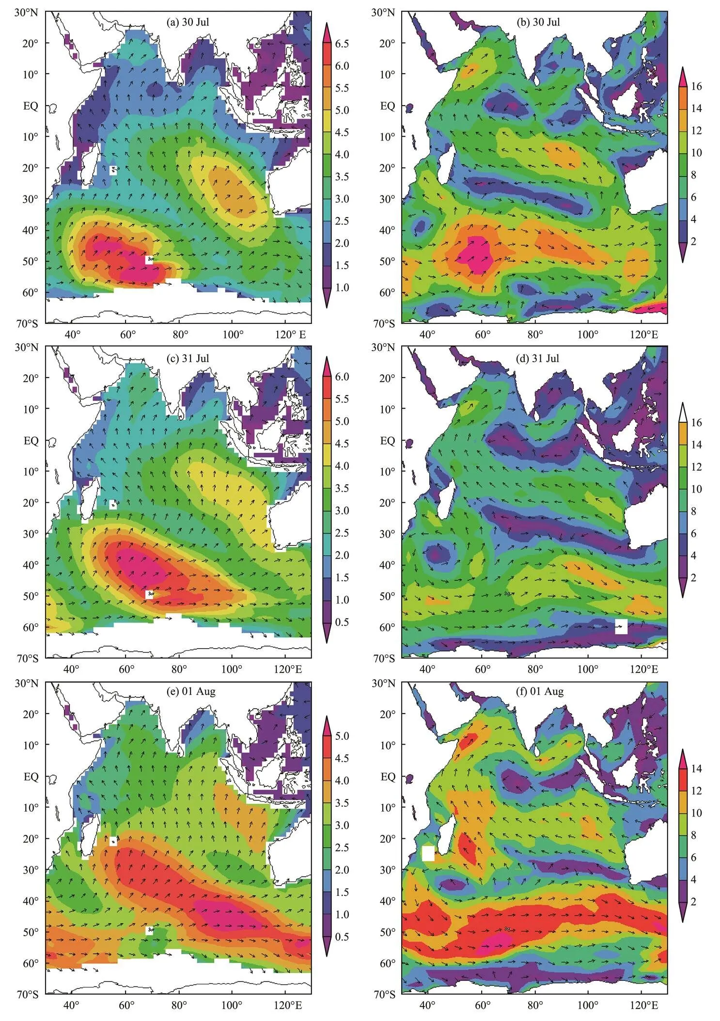
Fig.1 (a–f) Swell wave (left, unit: m) and sea surface wind (right, unit: ms−1) fields of the Indian Ocean in late July and early August of 2001.

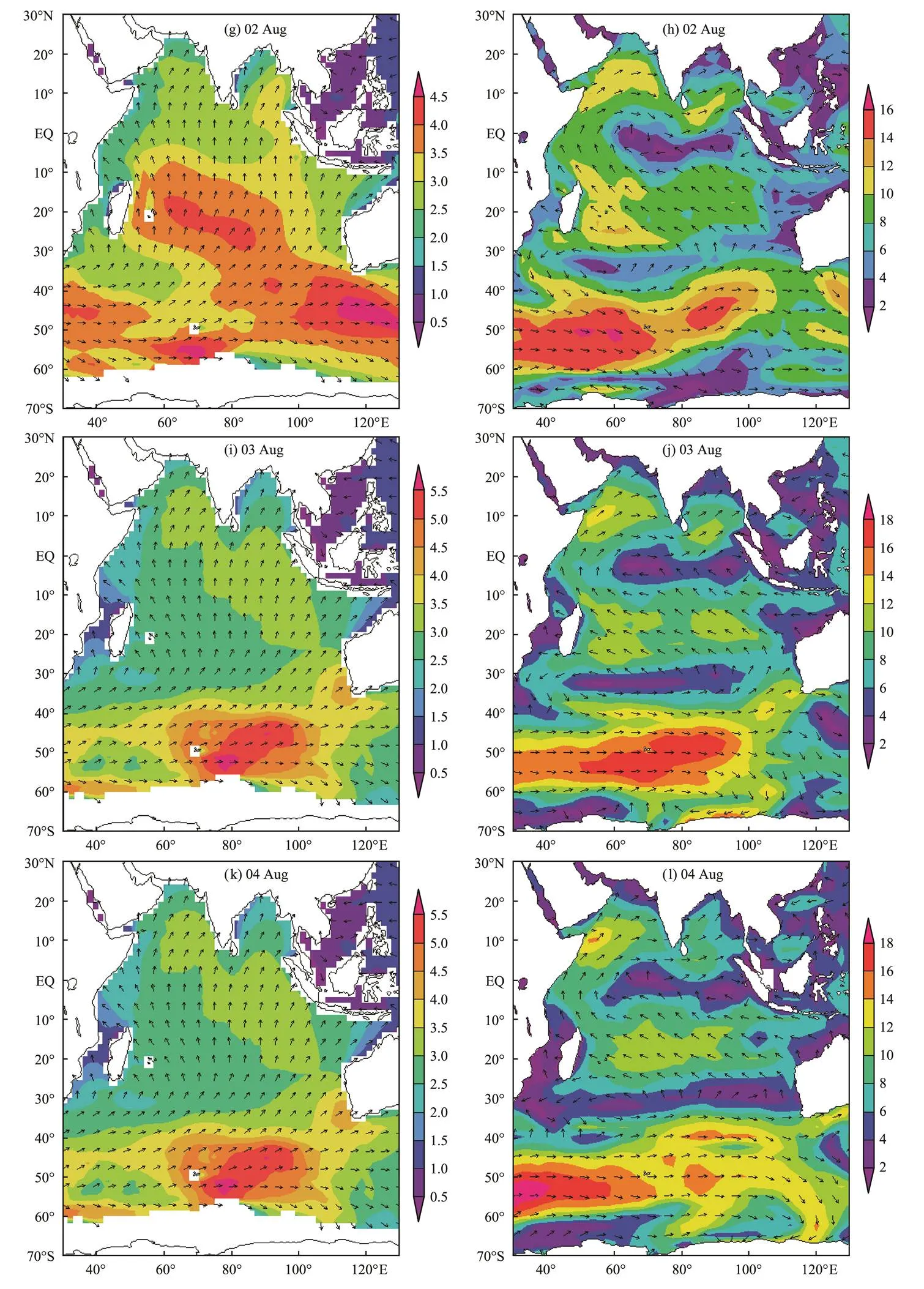
Fig.1 (g–l) Swell wave (left, unit: m) and sea surface wind (right, unit: ms−1) fields of the Indian Ocean in late July and early August of 2001.

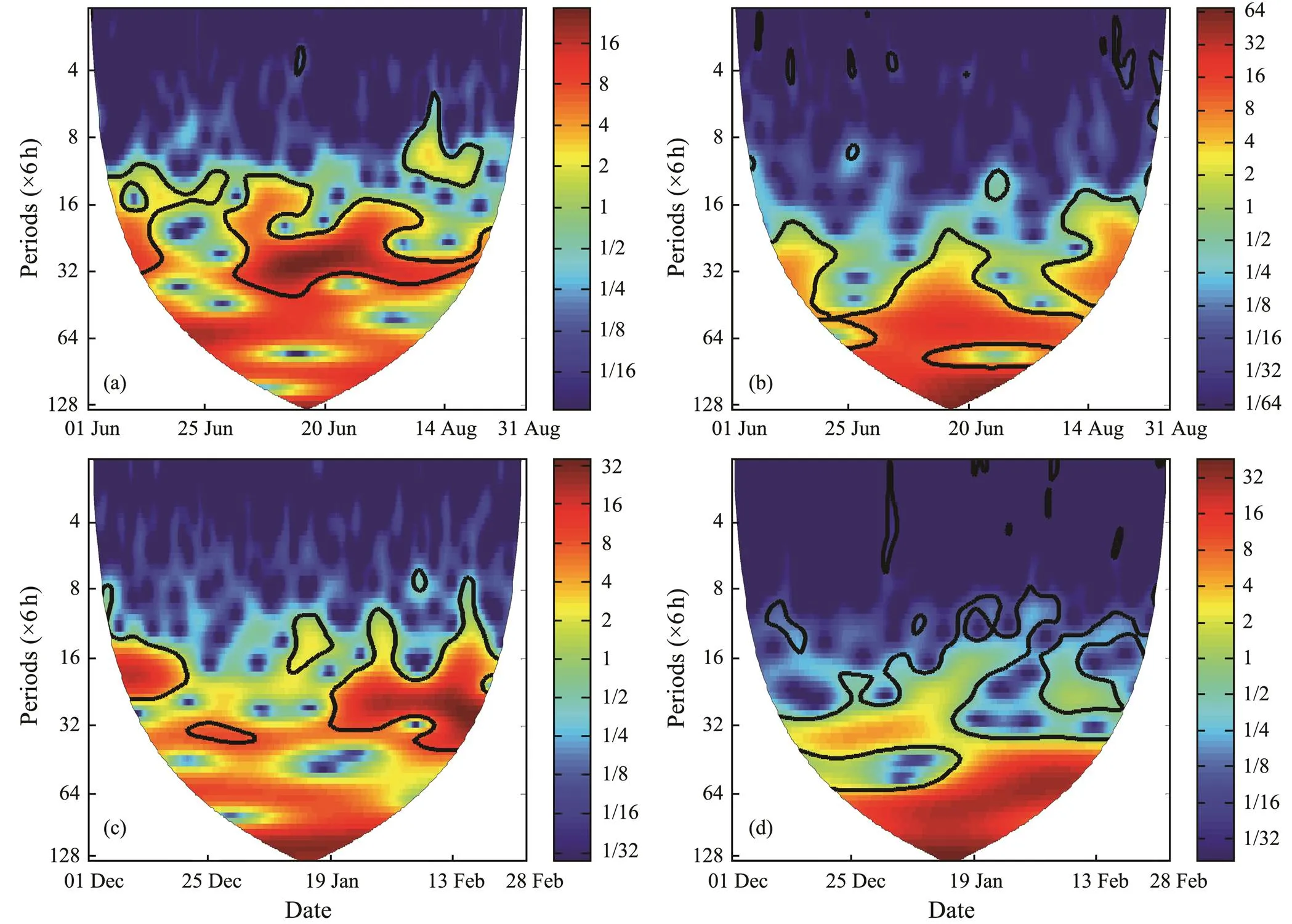
Fig.2 Wavelet analysis of SIWI (a, c) and IOSDEI (b, d) in JJA (a, b) and DJF (c, d) in 2001. Areas within the black solid line reflect significant periods.

Fig.3 Wavelet analysis of IOSDEI in JJA (a, b) and DJF (c, d) in 1990 and 1995.

3.3 Seasonal Correlation Between the Westerly Strength and the Range of Swell Diffusion

The SIWI and IOSDEI curves in JJA and DJF 2001 are plotted, as shown in Fig.4, to analyze the correlation between the intensities of the SIWI and IOSDEI. In JJA and DJF, the trends of the SIWI and IOSDEI curves are similar, and the SIWI leads the IOSDEI. The leading and lag-ging 30-interval correlations between the two parameters are calculated quantitatively, as shown in Fig.5, to analyze whether a leading or lagging correlation exists between the SIWI and IOSDEI accurately. In JJA, the correlation shows a peak value when the SIWI leads by 3 days (correlation coefficient [CC]=0.57, significant at the 99.9% reliability level). In DJF, the correlation reaches a peak value when the SIWI leads by 1.8 days (CC=0.46, significant at the 99.9% reliability level). We plot the 3-day leading SIWI and IOSDEI curves in JJA and the 1.8-day leading SIWI and IOSDEI curves in DJF and obtained good consistency between the leading SIWIs and IOSDEIs. This good agreement is also observed in JJA and DJF in the years 1990, 1995, and 2000, thus ruling out contingency for the consistency between the leading SIWI and IOSDEI.

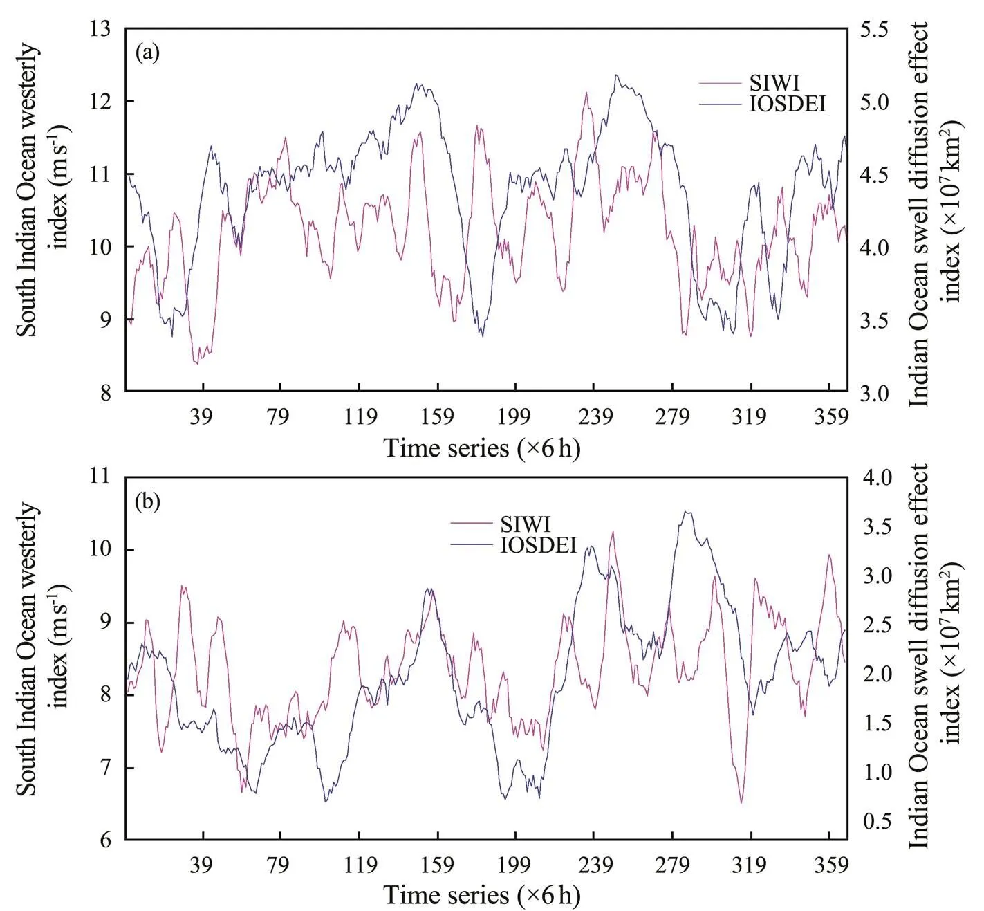
Fig.4 Six-hourly SIWI and IOSDEI in JJA (a) and DJF (b) in 2001.

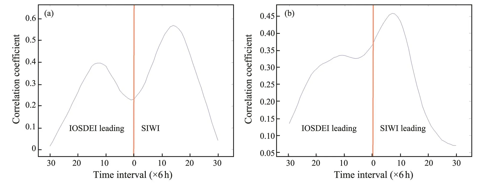
Fig.5 Leading and lagging correlations between the SIWI and IOSDEI in JJA (a) and DJF (b) in 2001.

3.4 Monthly Variations in the Correlation Between Westerly Intensity and Swell Diffusion

As shown in Fig.5, the CC between the SIWI and IOS- DEI in JJA 2001 is higher than that in DJF of the same year. The characteristics of the monthly variation of CCs between the SIWI and IOSDEI in different decades are also calculated. First, the leading and lagging 30 intervals between the SIWI and IOSDEI in January 1958 are calculated. The same method is employed to calculate leading and lagging CCs between the SIWI and IOSDEI in each month for the period of September 1957–August 2002. Then, the multiyear average CC in January for the period 1960–1969 is obtained. Similarly, the multiyear average CC in each month for the period 1960–1969 is obtained. Using the same method, leading and lagging CCs between the SIWI and IOSDEI in each month for differentdecades(1960–1969,1970–1979,1980–1989,and 1990–1999) are calculated, as shown in Fig.6. Regardless of the interval considered, the SIWI clearly leads the IOS- DEI in each decade, especially from October to March of the next year. Moreover, the CC reaches its peak value, even exceeding 0.4 (significant at the 99.9% reliability level), when the SIWI leads by 2.5 days.

For the period 1960–1969, the CC is lower in July than in other months. In addition, compared with those in other months, the CCs in February and November are the highest, and the CC peaks at up to 0.5 when the SIWI leads in 8 intervals (2 days). For the period 1970–1979, the CC is lower in July–September than in other months, but higher values are observed from October to March of the fol- lowing year. The CC peaks when the SIWI leads in 8–10 intervals (2–2.5 days). For the period 1980–1989, the CC is lower in April–May and in August–October than in other months. The CC peaks when the SIWI leads in approximately 10 intervals (2.5 days) in January–March and November–December and in 14 intervals (3.5 days) in June–July. For the period 1990–1999, the CC is low from May to September; the CC is highest in November–December and then in January–April, during which the SIWI leads in 8–14 intervals (2–3.5 days). The CC in JJA is clearly lower than that in all other seasons, and the CC is the highest in DJF in each decade.

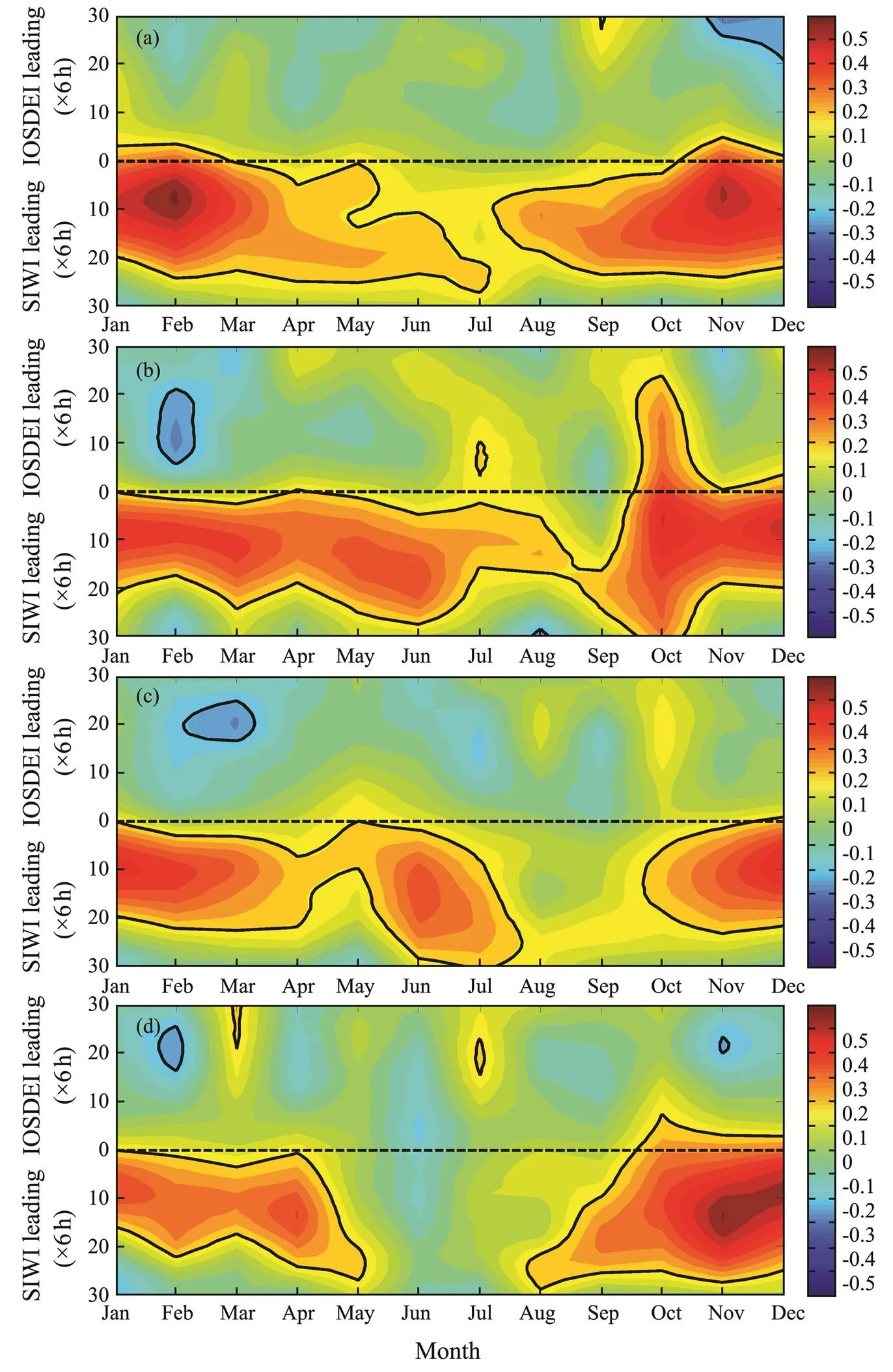
Fig.6 Leading and lagging correlations between the SIWI and IOSDEI for the periods 1960–1969 (a), 1970–1979 (b), 1980–1989 (c), and 1990–1999 (d).

3.5 Phase Relationship Between Westerly Intensity and Swell Diffusion

Figs.5 and 6 quantitatively exhibit leading and lagging correlations between the SIWI and IOSDEI. Here, cross wavelet analysis is used to find the leading and lagging correlations between the SIWI and IOSDEI in a common period, as shown in Fig.7.

In JJA (Fig.7a), in early and mid-June (1st to 100th intervals), the SIWI and IOSDEI have a common cycle of 4–8 days, during which the SIWI leads by approximately 3/4 phase (, 3–6 days). In early and mid-July (120th to 220th intervals), the SIWI and IOSDEI have a common cycle of 8–16 days, during which the SIWI leads by approximately 3/8 phase (, 3–6 days). In late July and August (220th to 360th intervals), the SIWI and IOSDEI have a common cycle of 8 days, during which the SIWI leads by approximately 3/8 phase (, approximately 3 days). Overall, the results in Fig.7a are fairly consistent with those shown in Fig.3a.

In DJF (Fig.7b), in December and January (1st to 240th intervals), the SIWI and IOSDEI have a common cycle of 8 days, during which the SIWI leads by approximately 1/4 phase (, approximately 2 days). In February (250th to 360th intervals), the SIWI and IOSDEI have a common cycle of 4–8 days, during which the SIWI leads by approximately 3/8 phase (, 1.5–3 days). In January, the SIWI and IOSDEI have a relatively long common period of over 16 days. During this common period, the SIWI leads by approximately one phase. These results show that the SIWI and IOSDEI have quasi-week oscillations in JJA and DJF. Fig.1 also illustrates that the formation process of a large swell in the South Indian Ocean westerlies and the extension and contraction area range of swell diffusion have a common period of 1 week, which is consistent with the results of the cross wavelet analysis. In addition, the SIWI is 2–3 days ahead of the IOSDEI during the common period of a quasi-week.

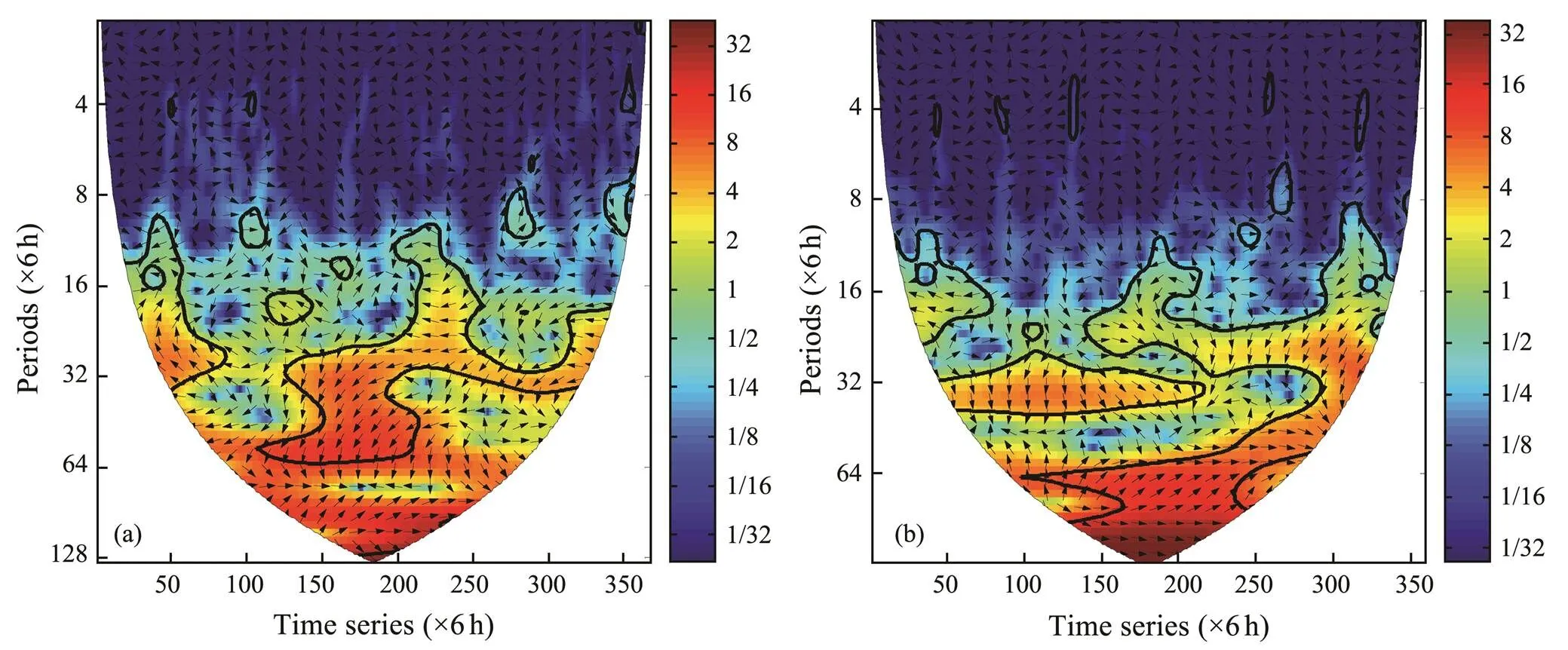
Fig.7 Cross wavelet transform analysis of the SIWI and IOSDEI in JJA (a) and DJF (b).

4 Conclusions

The 6-hourly south SIWI and IOSDEI are defined on the basis of ERA-40 wave reanalysis data, and the impact of the South Indian Ocean westerlies on the propagation of swell acreage is analyzed. The results show the following:

1) Swells generated in the South Indian Ocean mainly propagate from southwest to northeast. The swells propagate to the Arabian Sea when arriving at low-latitude waters, and the 2.0-meter contour can reach northward to Sri Lanka waters.

2) The size of the IOSDEI is mainly determined by the strength of the SIWI. This correlation peaks when the SIWIleads by approximately 2–3.5 days, which means the IOS- DEI needs approximately 2–3.5 days to fully respond to the SIWI. The CCs between the IOSDEI and SIWI show obvious seasonal differences at different stages over the past 45 years. The lowest CC is observed in JJA, while the highest CC is found in DJF.

3) In JJA, the SIWI leads by approximately 1/2–3/4 phase compared with the IOSDEI in their common cycle spanning 4–8 days. In addition, a common cycle of over 8 days is observed in JJA, during which the SIWI leads by approximately 3/8 phase. In DJF, the SIWI leads by approximately 1/4 phase in the common cycle of 4–8 days. A common cycle of over 12 days in the middle DJF, during which the SIWI leads by approximately 1 phase, is also noted. Thus, the SIWI and IOSDEI have common periods of approximately 1 week in JJA and DJF, over 8 days in JJA, and over 12 days in DJF. In the common period of the quasi-week, the SIWI leads the IOSDEI by approximately 2–3 days.

Acknowledgements

This work was supported by the National Key R&D Program (No. 2017YFC1405103), the Joint Funds of the National Natural Science Foundation of China (No. U1706220), the National Natural Science Foundation of China (Nos. 41901006, 41471005, and 41271016), and the Natural Science Foundation of Shandong Province (No. ZR2019BD005). The authors would like to thank the ECM- WF for providing the wave data and the anonymous reviewers for providing excellent suggestions to improve this manuscript.

Alves, J. H., 2006. Numerical modeling of ocean swell contributions to the global wind-wave climate.,11: 98-122.

Ardhuin, F., Chapron, B., and Collard, F., 2009. Observation of swell dissipation across oceans., 36: L06607, DOI: 10.1029/2008GL037030.

Caires, S., and Sterl, A., 2005. Validation and non-parametric correction of significant wave height data from the ERA-40 reanalysis., 22: 443-459.

Chen, G., Chapron, B., Ezraty, R., and Vandemark, D., 2002. A global view of swell and wind sea climate in the ocean by satellite altimeter and scatterometer., 19: 1849-1859.

Dong, B., Zheng, G., and Cong, P., 2009. Laboratory research on the influence of swell on wind wave energy., 39 (3): 381-386 (in Chinese with English abstract).

Liang, B. C., Liu, X., Li, H. J., Wu, Y. J., and Lee, D. Y., 2016. Wave climate hindcasts for the Bohai Sea, Yellow Sea, and East China Sea., 32 (1): 172-180.

Liu, J., and Yu, M., 1998. Characteristics of wind wave field and optimum shipping line analysis in North Indian Ocean., 17 (1): 17-25.

Mei, Y., Song, S., and Zhou, L., 2010. Interannual variation characteristics of wave field and wind field in the North Indian Ocean–South China Sea., 2 (5): 27-33.

Munk, W. H., Miller, G. R., Snodgrass, F. E., and Barber, N. F., 1963. Directional recording of swell from distant storms., A255: 505-584.

Samiksha, S. V., Vethamony, P., Aboobacker, V. M., and Rashmi, R., 2012. Propagation of Atlantic Ocean swells in the North Indian Ocean: A case study., 12: 3605-3615.

Semedo, A., 2010. Atmosphere-ocean interactions in swell dominated wave fields.. Acta University Upsaliensis, Uppsala, 53pp.

Semedo, A., Sušelj, K., Rutgersson, A., and Sterl, A., 2011. A global view on the wind sea and swell climate and variability from ERA-40., 24: 1461-1479.

Sterl, A., and Caires, S., 2005. Climatology variability and extrema of ocean waves–The web-based KNMI/ERA-40 wave atlas., 25: 963-977.

Yan, Z. D., Liang, B. C., Wu, G. X., Wang, S. Q., and Li, P., 2020. Ultra-long return level estimation of extreme wind speed based on the deductive method., 197: 106900.

Zhang, X., Liu, J. F., Zhang, X. H., Zhang, G. Y., Yang, L., and Yan, M., 2003. Annual variation analysis of sea wave field in the South Indian Ocean., 22 (2): 25-31.

Zheng, C. W., 2018. 21st Century Maritime Silk Road: Wave energy evaluation and decision and proposal of the Sri Lankanwaters., 39 (4): 614-621.

Zheng, C. W., Li, C. Y., and Li, X., 2016. Temporal and spatial distribution of wind sea, swell and mixed wave in Indian Ocean., 17 (4): 379-385.

Zheng, C. W., Li, C. Y., and Pan, J., 2018. Propagation route and speed of swell in the Indian Ocean., 123: 8-21.

Zheng, C. W., Zhou, L., Huang, C. F., Shi, Y. L., Li, J. X., and Li,J., 2013. The long-term trend of the sea surface wind speed and the wave height (wind wave, swell, mixed wave) in global ocean during the last 44a., 32 (10): 1-4.

# These authors contributed equally to the work.

. E-mail: chinaoceanzcw@sina.cn

July 9, 2019;

January 8, 2020;

March 26, 2020

(Edited by Xie Jun)