Learning a Deep Predictive Coding Network for a Semi-Supervised 3D-Hand Pose Estimation

Jamal Banzi, Member, IEEE, Isack Bulugu, and Zhongfu Ye

Abstract—In this paper we present a CNN based approach for a real time 3D-hand pose estimation from the depth sequence.Prior discriminative approaches have achieved remarkable success but are facing two main challenges: Firstly, the methods are fully supervised hence require large numbers of annotated training data to extract the dynamic information from a hand representation. Secondly, unreliable hand detectors based on strong assumptions or a weak detector which often fail in several situations like complex environment and multiple hands. In contrast to these methods, this paper presents an approach that can be considered as semi-supervised by performing predictive coding of image sequences of hand poses in order to capture latent features underlying a given image without supervision. The hand is modelled using a novel latent tree dependency model(LDTM) which transforms internal joint location to an explicit representation. Then the modeled hand topology is integrated with the pose estimator using data dependent method to jointly learn latent variables of the posterior pose appearance and the pose configuration respectively. Finally, an unsupervised error term which is a part of the recurrent architecture ensures smooth estimations of the final pose. Experiments on three challenging public datasets, ICVL, MSRA, and NYU demonstrate the significant performance of the proposed method which is comparable or better than state-of-the-art approaches.

I. Introduction

HAND pose estimation from depth is the first step for numerous computer vision applications. It has been widely applied to human-machine interaction (HMI), since it provides the possibility for future multi-touchless interfaces.An accurate hand pose estimation provides a natural way of interaction between human and virtual space that achieves greater user experience. The conventional human-machine interactions are limited to 2D plane display, and are only suited where users sit behind the computing devices. In contrast to conventional HMI, hand pose estimation offers 3D user interaction without direct contact with the computing device, and provides a possibility for the new interface leading towards seamless human-computer interaction see Fig.1.

Fig.1. An example of 3D-hand pose estimation.

Indeed, there are significant numbers of literatures devoted to developing fast and accurate hand pose estimation systems thanks to the advent of low-cost depth sensors [1]–[5].However, the state-of-the-art methods for 3D-hand pose estimation from depth rely heavily on large numbers of depth images annotated with hand joints [6]–[10]. These methods have demonstrated promising results using deep learning approaches [11]–[15] which are all fully supervised.

Nevertheless, precise annotation of 3D hand joints on real data is difficult to come by and time-consuming. Additionally,the computation complexity of the annotation process increases the chance of generating multiple residual errors[16]–[19]. This reduces the utility of deep neural networks on hand pose estimation domain.

In addressing the challenge of dense annotation of the hand data, this paper presents a deep neural network algorithm with a predictive coding model (Deep PCM) that can predict hand joint positions recursively using deep recurrent convolutional networks with bottom up and top down connections in a semisupervised fashion. Prior to joint prediction, the hand is modeled using latent dependency tree model (LDTM), which improves hand detection with much better accuracy, discussed in detail in Section II. The generated hand topology is fed into Deep PCM, and then encoded to generate a hand representation which will be mapped with the decoded depth maps. Finally, the joint regression is performed by training end to end pose estimator based on depth images. The included unsupervised error vector, provides an error correction population used to improve estimation accuracy of the final hand pose.

The gist of this paper can be summarized as follows:

1) A new way of modelling a hand topology using LDTM which transforms internal joint locations to an explicit hand representation. This hand representation is more compact and invariant in scale and view angles.

2) Unlike previous methods which only focus on pose estimation based on strong assumptions (that the hand is the nearest object from the camera) or relying on a weak hand detector, we model the hand topology using LDTM and integrate it with the pose estimator into one pipeline.Therefore, our hand pose estimation is based on the prior knowledge of the human hand.

II. The Proposed Approach

This section explains in details about the whole process of hand joints position estimation from the given hand depth.Ideally, we formulate the hand topology of a human hand using a novel LDTM. Then, we use data-dependent method[11], [20] to jointly learn LDTM which generates latent variables of the posterior pose appearance, and deep PCM which generates pose configuration. We learn the mapping between the two individual domains. Eventually, the complete network is trained end to end for the pose estimation process as in many literatures [21]–[27].

A. Representation of a Hand Topology

We leverage LDTM to represent hand topology. This is indeed a viable choice because LDTM models dependencies between random variables with a structure that can change dynamically based on the variable values. It is therefore capable of modeling context-specific independencies.

The LDTM encodes the relation between variables with a dependency tree. A distribution over all possible dependency trees given the current assignment of variables is specified using a first-order non-projective dependency grammars (DG)as in [28]–[30]. The probability of a complete assignment can then be computed by adding up weights of all the dependency trees. Fig.2 shows an example of using LDTM to compute joint probability of the assignment of a given variable. The number of possible branches grows exponentially with the number of variables, but the summation of trees weights can still be computed tractably by utilizing the Matrix-Tree

Fig.2. An example of using LDTM to compute joint probability.

Theorem.

These three joints are more reliable and are chosen as the foundation to construct trinary nodes. X1and X2are variables which form a pairwise dependency VnXn. Each dependency has a weight which is used to grow a tree and calculate the probability of joint distribution.

The LDTM hand topology is presented in Fig.3.

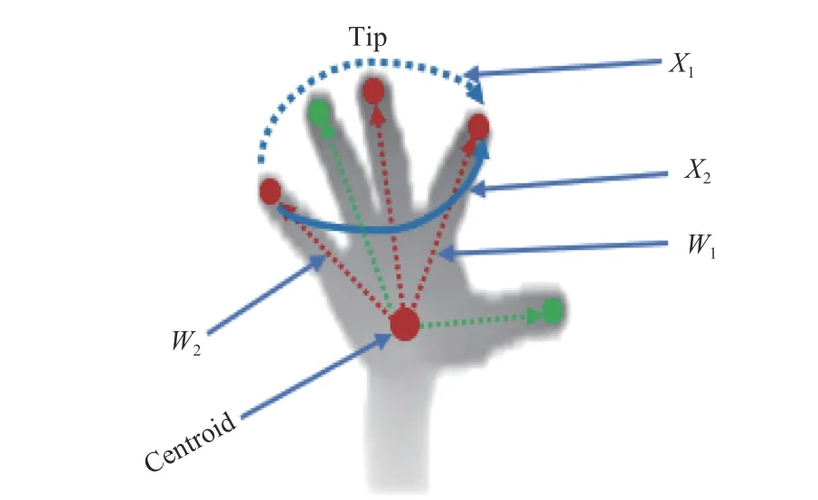
Fig.3. LDTM representing a hand model geometry.

In contrast with the traditional LTM [30], [31] models, the LDTM has the following unique features:

1) LDTM models the latent dependencies between random variables, i.e., dependencies are dynamically determined based on the assignment of random variables.

2) LDTM considers all possible tree structure at the same time resulting in easier learning.

3) LDTM removes all possible latent node dependencies,and hence improves hand joint detection as shown in Fig.3.

B. Learning the Hand Topology

An LDTM is a tree-structured graphical model where leaf nodes are observed, and internal nodes can either be observed or latent as for the conventional latent tree model, but further LDTM encodes relations between variables with a dependency tree. We denote the LDTM tree model as

where the vertices are composed of observable vertices X1,and latent vertices X2= {x2}, where x2⊆X2; and V denotes pairwise dependencies among variables. We assume that the strength of each pairwise dependency is independent and denote the dependency strength from node xiand node xjby an edge weight wijas in [30]. The distance matrix that defines the distance function of an LTM and LDTM is presented in Fig.4. The information distance matrix results show that LDTM could cover all 21 vertices and 1 centroid necessary for Chow-Liu neighbor joint (CLNJ), whereas LTM covers only 17 vertices.

C. Edge Weight Function

The partition function Fxis the sum over the weights of all possible dependency trees for a given assignment x, which represents the weight of the assignment. It is given as

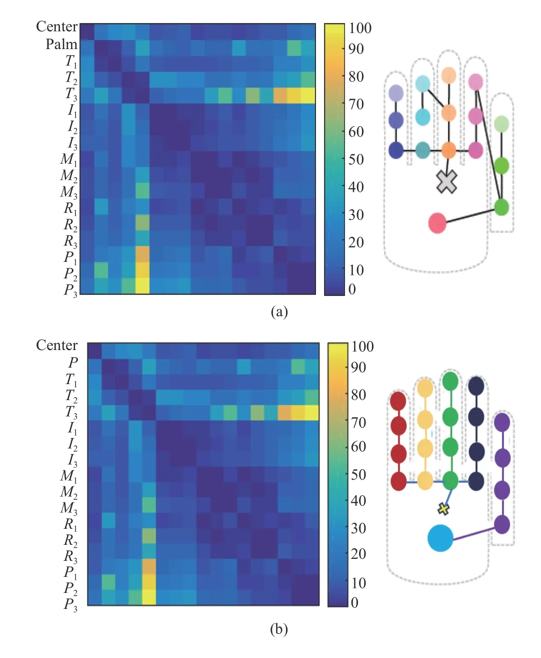
Fig.4. (a) Distance matrix generated with the LTM. T: thumb; I: index; M:middle finger; R: ring finger; P: pinky. The subscript numbers represent: 1:proximal phalanx; 2: intermediate phalanx; 3: distal phalanx; (b) Distance matrix generated with the LDTM.

where S is a spinning tree, S(Nx) is a set of all possible dependency nodes. LDTM requires that the weight of each dependency (xi,x2) is the conditional probability. Therefore,the vertices X1and X2are given assignment X1= xior the root node and its probability is given as wxj/xisuch that 0 ≤wxj/xi≤1. For all nodes, there are given assignment,x=(x1,x2,...,xn), which are generated recursively in a topdown manner. We grow a tree with n+1 nodes uniformly at random. The root node is given as x0. Then starting from this root node, we recursively traverse the tree in pre-order such that at each non-root node, a variable to value pair is generated conditioned on the variable to value pair of its parent node. The whole process is summarized in Algorithm 1.The probability of generating an assignment x is given as

where C is constant, representing the uniform probability of the tree structure. α is constant with respect to x.

Note that some variables may be assigned to multiple nodes and therefore there might be missed variables. However, since the focus is only for the node space of the valid assignments,i.e., no redundancy nor missing variable assignment, we define the joint probability of a valid assignment x as

where A is the set of valid assignments and γ is the normalization factor.

D. Unsupervised Learning

We describe our algorithm to learn LDTM from the depth where the dependency structure of each training instance is unknown. For each internal node as in the Chow-Liu tree [31],a recursive joining method scheme is applied by identifying its neighborhood.

This method can produce consistent LDTMs without redundant latent nodes. Applying log-likelihood to the function given in (3), we obtain

Algorithm 1 LDTM topology Input; A set of training sample S,T =F(X1 ∪X2,Xn) a pre-learned LDTM, Output; LDTM topology Procedure, Grow (S, T)Divide S into corresponding subset S0,…,Sn Let i = 0, j = 0, initialize ith node of LDTM and its forest jth Let d = 0(i,j,So,n) SPLIT Function SPLIT Select a set of split candidates If the number of chosen samples is sufficient then Save j as a split node into T i ∈X2(i,j,S,n) Else if then Save j as a partition node into T S =S ∪Sd+1 Let SPLIT Else Save j as leaf node into T Return End i,j,S,d+1

D={xn}n=1|D|

Where is the training sample.

It is noticeable that the log-likelihood is computed on p(x),the probability of generating an assignment, and not of φ(x),the probability of a valid assignment. This makes our learning algorithm tractable, and also encourages the learned model to be more likely to produce valid assignments.

III. Deep PCM Network

We present the deep learning architecture with the predictive coding model for prediction and subsequent regression of hand joint positions in Fig.5. A predictive coding [32]–[34] is an RNN with the following features:

1) The start time, holds t0=0, while τ=1, and τ is constant.

2) The initial input state S0of a time series constitutes the initial components of the start vector x0.

3) It has linear activation applied to all neurons.

4) The initial weight Winand relative weights Wreare random, independent, and identically distributed from the

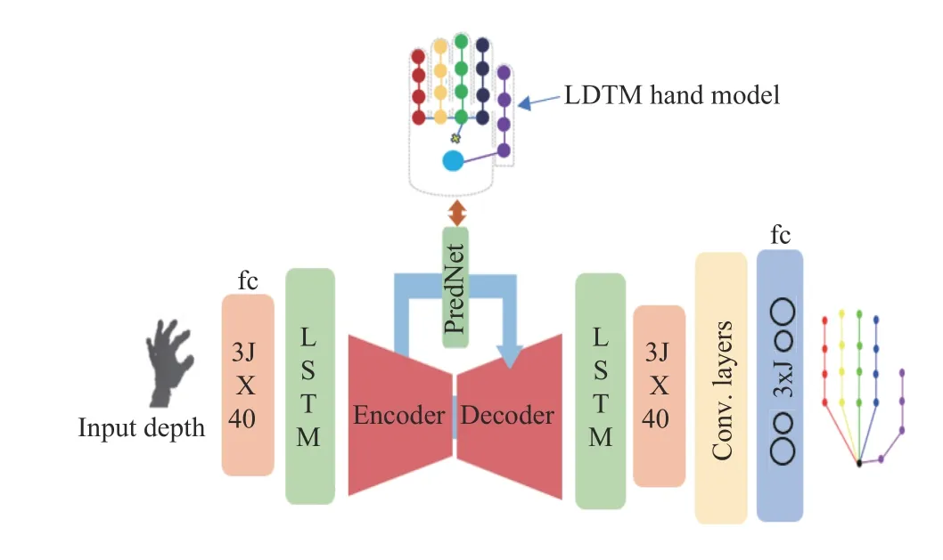
Fig.5. Overview of the proposed system showing the network architecture.Fc stands for fully connected layers and conv. stands for convolutional layers.

Wout standard normal distributions, whereas the output weight is learned.

5) The input and output are arbitrarily connected and there is no clear distinction between them.

A. Operation of Predictive Coding Network

The autoencoder learns the low-level representation of the sequenced image data, which will then be deformed,compressed and projected by the decoder to form an actual input.

The sequence is read by the LSTM step by step and encode the input sequence to model an internal representation of the entire input sequence as a fixed length vector which is then passed to the PredNet. Upon receiving, the PredNet makes a local estimation.

These local estimations are subtracted from the actual input and passed along to the next layer and finally to the fully connected layer where joint positions are regressed.

Basically, each module of our network consists of four basic deep layers:

1) An input convolutional layer ( Pi);

2) An estimation (prediction) layer (Pl);

3) An error regression layer (El);

4) A recurrent representation layer (Rl).

For representation neurons, we explicitly use convolutional LSTM units [35]. This is a recurrent convolutional layer responsible for the generation of estimations from the input layer.

B. Long Short-Term Memory (LSTM)

LSTM model correlation between observed and hidden state with a memory unit. This provides significant improvement over RNNs. We apply LSTM to extend our predictive coding with two advantages. Firstly, induce the memory information.

Secondly, handles sequential data better and avoids the gradient vanishing problem. We show how LSTM handles the vanishing problem and perform backpropagation error as in[35]. The core idea of LSTM is to encode the information of the inputs ( xtand yt−1) that has been thrown away from the cell state Ctand output of yt. Further LSTM has gates which control states with a sigmoid function. These are forget gate ft, input gate it, output gate ot, and modulation gate gt.Therefore, for a given image sequence {x1,...,xT}, we have the following gate definitions:

As for RNN, to make a prediction, we add a linear model over the hidden state ht, and output the likelihood with SoftMax function.

Given ground truth at time t as ytwe can minimize the least square (yt−zt)2/2 to estimate hand parameters.

Hence, for the top layer classification, with weight Wz, we now take derivate with respect to zt, and i,j,S,d+1,respectively.

where the gradient is considered only with respect to hT.However, for any time step t its gradient will differ a little, see(15) below:

This will then be back propagating it with every time step t.

C. Error Regression Scheme

Fig.6. Illustration of the data flow within our predictive coding network(PredNet).

The update of state is presented in Algorithm 2.

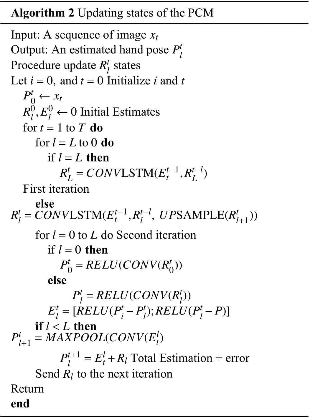
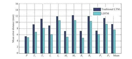
Algorithm 2 Updating states of the PCM Input: A sequence of image xt Output: An estimated hand pose Rtl Ptl Procedure update states i=0, and t=0it Let Initialize and Pt0 ←xt R0l,E0l ←0 Initial Estimates do for l=L to 0 do if l=L then RtL=CONVLSTM(Et−1t ,Rt−lL ) for t=1 to T First iteration else Rtl=CONVLSTM(Et−1t ,Rt−ll , UPSAMPLE(Rtl+1)) do Second iteration if l=0 then Pt0=RELU(CONV(Rt0)) for l=0 to L else Ptl=RELU(CONV(Rtl))Etl =[RELU(Pti −Ptl);RELU(Ptl −P)] if then Ptl+1=MAXPOOL(CONV(Elt)l

IV. Experiment

We perform a complete experiment to unveil the performance of the proposed approach.

A. Experimental Settings

The Model was implemented with the python library, using Theano [36] and Keras. The model parameters are optimized using gradient descent Adam algorithm [32] with all parameters set to default values.

B. Data Pre-Processing

Before the training stage, we first need to pre-process the raw data from the dataset. The input of the pose estimator is the cropped image, but the original ground truth of the image is the absolute position in the entire raw image. Therefore,there is a need to first transform the ground truth into a relative position with respect to the center of the hand. Finally,the images are sized to 96 × 96 and in grey-scale with values normalized between 0 and 1.

C. Regressive Training

We train our Deep PCM regressively with the learning time gradually decreased.

The model was based on the pre-trained model [37] and was trained to predict hand joints position. The loss was taken as the sum of the firing rates of the error neurons in the zeroth pixel layer. A random hyperparameter search was performed over fourth- and fifth-layer models of the posterior position.

Our model consists of 5 layers with 3 by 3 filter sizes of all convolutions and stack size per layer of (1, 32, 64, 64, 128,256). The initial training rate is set to 0.001 dropped by learning ratio of 10 after every 60 epochs. The general implementation specification of the proposed system is presented in Table I.

TABLE I Implementation Specification of Our System

V. Evaluation of the Proposed Approach

This section discusses the comparison of our approach with the existing state-of-the-art approaches. We evaluate the performance of our approach on three publicly available datasets for hand pose estimation: The NYU datasets [21],ICVL dataset [38], and MSRA dataset [15]. Table II below presents the details of the datasets used.

TABLE II Datasets Used for Evaluation of the Proposed Method

A. Evaluation Criteria

We report the values stated in papers or measured from the graphs if provided, and or plot the relevant graphs for comparison. We use two different commonly used criteria to evaluate our method, namely:

1) The fraction of sample error distance within a threshold.Here we measure the fraction of success frames whose error distance of each joint is less than a certain threshold.

This is the most challenging evaluation criterion since the single mistaken joint may decline the judgment of the entire hand pose.

2) Mean error distance of different joints and their average.This is recognized as the most commonly used criteria in the literature of hand pose estimation and allows comparison with many contending baselines, because of the simplicity of the evaluation.

B. Self-Comparisons

We firstly evaluate the impact of modeling hand topology using LDTM. We utilize NYU datasets to depict the number

Fig.7. Self-comparison showing the performance of LDTM. Left: the success rate of the hand detection part of two methods; Right: the error rate of the two methods of modeling a hand.

Fig.8. Effect of LDTM and LTM on the mean error distance of each joint.

Fig.9. Comparison with the state-of-art on ICVL [38] (left); NYU [21] middle; MSRA [15] right. It shows the fraction of samples whose distance between all estimated joints and ground truth is less than a certain threshold.

of success frame over a certain threshold. Illustrated in Fig.7,the impact of LDTM based hand topology on the estimated joints is presented. The experiment shows that LDTM performs better than the traditional LTM. Also, the proportion of success frame is higher with the LDTM than both LTM and the assumption-based method. Using ICVL dataset, we present standard evaluation metric of mean error in mm for each joint across the sequence in Fig.8. LDTM consistently performed better with minimum error to all joints. This experiment shows that using accurately modeled hand topology, increases accuracy of estimation of the pose,indicating the effectiveness of using LDTM and that it can be applied to real time applications.

We first measure the proportion of good frames over a certain error threshold using Criteria 1 and present results in Fig 9. Empirical results show that our method outperformed many of the contending approaches by a large margin while it works comparably with few methods that have attained state of art results. The reason for this superiority is attributed by the following. Firstly, a strong hand topology based on a novel LDTM which is capable of modeling context-specific independencies, and therefore estimation of the final hand pose is based on the prior knowledge of the hand representation. This is contrary to many of the existing approaches which are either based on the strong assumption that the nearest object behind the camera is the hand, or based on a very weak detector to detect a hand [44]–[46]. Secondly,the proposed approach has an intrinsic error regression technique which smooths the estimated values allowing the network to learn its own mistakes and fix them to finally increase the accuracy of estimation.

Fig.10. Comparison with the state of the arts on NYU [21] (left); ICVL [38] (middle); MSRA [15] (right). It measures the error distance of different joints and their average (P: palm; T: thumb; I: index; M: middle; L: little).

For example, on ICVL dataset [38], Fig 9 (left) when the error threshold is 20 mm, the proportions of good frames of our approach achieve 10% and 15% better than deep prior++[27] and Zhou et al. [39], respectively.

On NYU dataset [21], when the error threshold is between 20 mm and 30 mm the proportion of good frames of our method is comparable to deep prior++ [27], and 10% better than the CrossingNet [40]. On MSRA dataset [15], when the error threshold is between 20 mm and 30 mm, the proportion of good frames is comparable to PointNet [43], 5% better than deep prior++ [27] and 25% better than CrossingNet [40],BigHand [41], and Madadi et al. [42]. These results indicate that the proposed method is robust and can accurately estimate the location of the hand joint positions.

We also present the error distance of different joints and their average in Fig.10. The experimental results show consistent performance over all state-of-the-art methods on NYU and ICVL. However, on MSRA, PointNet [43]performed better than our method in overall mean error.Nevertheless, if the error distance of different joints is considered, we can see that our results are better than theirs for most of the significant joints.

VI. Conclusion

In this paper, we present a novel approach to model hand topology based on LDTM which captures hand latent features and observable features to construct hand joint representation.We integrate LDTM with the Deep PCM using a dataindependent method to encode the hand representations and then map with the decoded hand depth map. We then use the multi-layered convolutional neural network to regress a 3D hand pose. The predictive coding part of the network provides unsupervised learning of the image sequences, while the error term contends estimation errors by feed-forwarding every local estimation as an input of the subsequent network layer.As a result, our system can accurately estimate a hand pose based on the prior knowledge of the hand representation.