Control of water contamination on side window of road vehicles by A-pillar section parameter optimization ＊

Li Xin, Xing-jun Hu, Jing-yu Wang

State Key Laboratory of Automotive Simulation and Control, Jilin University, Changchun 130025, China

Abstract: The water contamination on the side windows of moving vehicles is a crucial issue in improving the driving safety and the comfort. In this paper, an effective optimization method is proposed to reduce the water contamination on the side windows of automobiles. The accuracy and the efficiency of the numerical simulation are improved by using the lattice Boltzmann method, and the Lagrangian particle tracking method. Optimized parameters are constructed on the basis of the occurrence of the water deposition on a vehicle’s side window. The water contamination area of the side window and the aerodynamic drag are considered simultaneously in the design process; these two factors are used to form the multi- objective optimization function in the genetic algorithm (GA) method. The approximate model, the boundary-seeded domain method, and the GA method are combined in this study to enhance the optimization efficiency. After optimization, the optimal parameters for the A-pillar section are determined by setting the boundary to an area of W =7.77mm , L =1.27mm and H =11.22mm . The side window’s soiling area in the optimized model is reduced by 66.93%, and the aerodynamic drag is increased by 0.41% only, as compared with the original model.It is shown that the optimization method can effectively solve the water contamination problem of side windows.

Key words: Water contamination, aerodynamic drag, A-pillar section parameters, multi-objective optimization, approximate model,genetic algorithm

Introduction

The management of the water contamination on vehicle surfaces has increasingly gained attention in recent years[1]. Raindrop deposition on vehicle windows may form liquid layers and rivulet, to refract and block the light and to seriously impair the visibility of views for drivers. The early research of the water contamination focused on the control of the excessive rain on the windshields, leading to the application of the windscreen wipers. Other studies attempted to use the air curtains to prevent the water droplets from accumulating on the windshields, but these methods failed to be adopted in practical cases due to their high energy requirements and severe noise[2]. Lately, Goetz[3]designed an automatic wiper system based on the rain sensors to effectively control the water contamination on the windshields.

Numerous studies were recently conducted for the effect of the water contamination on the side window. The water accumulation on side windows comes roughly from three different sources: the rain droplets captured directly by the free flow hit, the water on the windshield flows through the A-pillar under the combined action of the wipers and the airflow, and the water caught by the rear mirrors and its breakup from this vehicle component[4]. Various studies of the three sources focused on a single component, such as the rear mirror or the A-pillar.Waki et al.[5]performed a wind tunnel test, including a photosensitive study, by focusing on the development of the liquid on a rear mirror and found that the water film breaks up into droplets at the edge of the mirror and moves with the airflow. Bannister[6]investigated the influence of various types of mirrors on the contamination patterns of the side window and analyzed the relationship between the mirror design and the side window soiling.

An optimization of the shape of the A-pillar, later proposed by Karbon, was shown to be highly effective in suppressing the water contamination on the side window[7]. It was shown that the water on the front windshield surface can flow over the A-pillar and move to the side windows under the action of the wipers and the airflow an A-pillar geometry modified by a wedge installation was also studied as a means to change the flow structures and the water film dynamics. It was shown that the water film could be easily separated from the A-pillar surface, to reduce the water movement along the edge of the A-pillar to the side window[8]. Further investigation showed that the movement of the water film was changed by the different surface shear stresses caused by the A-pillar modifications[9]. However, most of the attempts on the A-pillar optimization to solve the water contamination problems involve generally considerations of several shapes and then the comparison of their effects to select the best A-pillar design, thus, the results may not necessarily be optimal. Moreover, the different end outcomes depend heavily on the designers’engineering experience. Meanwhile, some unsuitable changes in the A-pillar shapes can lead to the boundary layer separation and the vortex formation,causing an increase of the aerodynamic drag[10].However, there are few studies of the balance between the water contamination and the aerodynamic drag.

In this study, numerical simulations are performed and an optimization framework is constructed for the design of the A-pillar section parameters and the investigation of the effect of the water contamination on the side windows. The simulations are based on the lattice Boltzmann method (LBM) and the Lagrangian particle tracking method. Moreover, the boundary seeded domain (BSD) method is adopted to improve the efficiency of the computation while guaranteeing the accuracy of the simulations. Then, an approximation model and the genetic algorithm (GA) method are combined to optimize the three section parameters for the A-pillar, and a multi-objective optimization function (the water distribution area Swand the aerodynamic drag coefficient Cd) is applied. Finally,the A-pillar shape of the optimal model is determined and compared with that of the original model. Figure 1 shows the flowchart to summarize the proposed aerodynamic and water contamination optimization process.

1. Numerical simulation

1.1 Modeling of the continuous phase

The numerical simulation, a technique widely used in the wind engineering, and the automotive aerodynamics simulations[11], is performed using the commercial software powerFLOW. The continuous phase is simulated with the LBM, a numerical method typically used for the flow field simulation based on the kinetic theory and the statistical mechanics[12]. The LBM is a special discrete format method used to solve continuous Boltzmann equations. Unlike the incompressible Navier-Stokes equation, the LBM treats the fluid as a group of particles that can be completely dispersed in time and space. The LBM can also describe a flow phenomenon based on the particle migration and collision. The lattice Boltzmann equation for the velocity and time discretizations can also be used to describe the particle evolution.

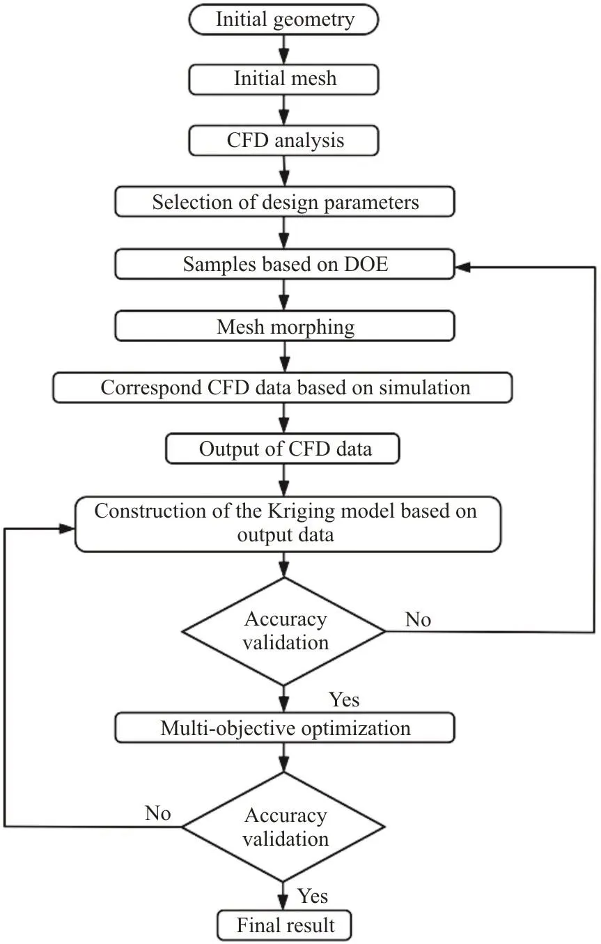
Fig. 1 Flowchart of the optimization process

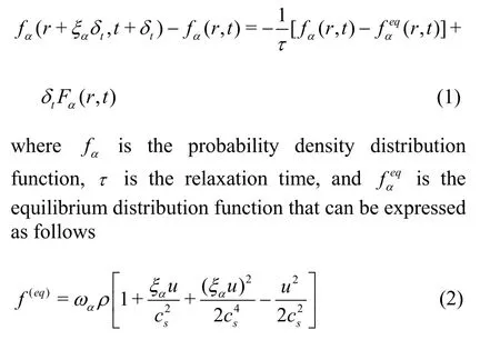
whereαω is the weight coefficient, ρ is the fluid density,αξ is the discrete velocity, u is the fluid velocity and csis the lattice sound velocity with a value of 1/3c. In this paper, we are confined to the lattice Boltzmann model in the three-dimensional space with D3Q19, and the parameters are selected as follows:

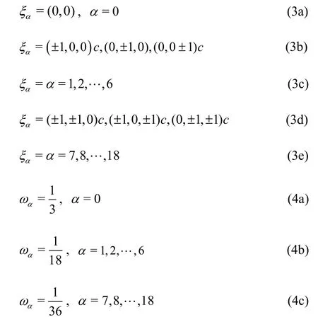
The resolvable scale flow of the turbulent fluid field is computed with the method called the very large eddy simulation. This method can be used to calculate the grid directly. And the sub grid scale can be described by using the RNG k-ε function.Moreover, this method can ensure the accuracy of the calculations of transient problems, such as the water management and the aerodynamic drag[13].

1.2 Modeling of water contamination

The Lagrangian particle model is integrated for the use of the LBM solver to allow for the two-way coupling between discrete and continuous phases.This approach is widely used in the calculation of many multiphase flow problems, such as the atmospheric pollutants[14], the wind-driven rain[15], and the pesticide sprays. This method can also contain models to describe the breakup of raindrops due to the aerodynamic share, the splashes, and the reentrainment of the drops from surfaces into airflows.The Taylor analogy breakup model is used to solve the droplet breakup, and the O’Rourke model is adopted to calculate the drop collision[16]. The trajectory of the particles in the flow field is tracked by solving a motion equation. The motion equation of a single raindrop particle can be expressed as follows[1]:

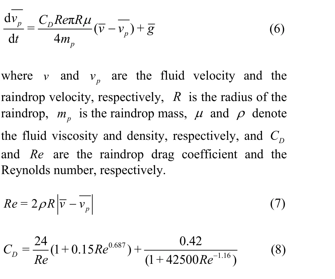
The surface film dynamics is simulated by using the thin film model. In this model it is assumed that the drops form a thin film of fluid, much smaller in thickness than the characteristic geometrical size of the vehicle’s wall. A film’s movement is known to be affected by the shear stresses acting on the air-liquid and liquid-solid interfaces[17]. Gravity, regarded a volume force of films, is treated as an influencing factor of the film’s motion[18].

1.3 Simulation of the continuous phase setting

The DrivAer model, with a genetic and detailed vehicle geometry based on the Audi A4 and BMW 3 series[19], is adopted in this study (Fig. 2). Compared with simplified models, such as Mira, Ahmed, and SAE models, the DrivAer model involves more exterior geometry features to narrow the gap between the idealized vehicles for the aerodynamic research and the realistic vehicles. The DrivAer model is widely used in many experimental and numerical investigations of aerodynamics studies[20]. An important advantage of using this model is that we can find the common phenomenon of vehicles. The side window area is divided into two regions of view, namely, (1)the main view region and (2) the secondary view region, and four measured points are selected to record the changes of the water film thickness.

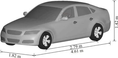
Fig. 2 Numerical calculation model

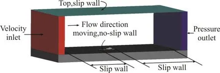
Fig. 3 (Color online) Computational domain and boundary conditions

Figure 3 shows the calculation domain. The boundary of the calculation domain is set far from the body surface to eliminate the effects of the simulation domain boundary on the surrounding flow field of the vehicle. However, the boundary space cannot be extremely large in view of the computational resources. Taking L to be the length of the vehicle,the computational domain is 21L long, 8L high and 14L wide. The front of the vehicle is located 9L from the inlet and the back of the vehicle is 11L from the outlet. The fluid enters the computational domain with a uniform velocity of 27.28 m/s from the inlet. The turbulent intensity at the inlet is prescribed as 0.5%, to match the wind tunnel environment. The density of the air is ρ and the dynamic viscosity of the air is μ , which are set as 1.205 kg/m3and 1.81×10-5Pa·s. For the fully developed vehicle wake, the outlet is set as the pressure outlet and the static pressure is equal to zero.The surface of the model is set as the no-slip wall boundary to simulate the actual driving state of the vehicle. The wheels are fixed, and the floor is set as the moving and no-slip wall boundary, with the speed equal to the fluid velocity to avoid the ground effects.The other components are set as the slip walls.

The surface elements of the vehicle are divided using the STL method to effectively preserve the vehicle’s features. The maximum surface mesh chord deviation is set as 0.0125 mm, and the maximum mesh size is 15 mm. The accuracy and the reliability of the simulation are ensured and the total number of grids in view of saving computational resources is controlled using ten grid refinement regions (Fig. 3).The minimum voxel size is set as 1.25 mm and used in the regions of largest pressure gradient, such as the A-pillar and the bonnet leading edge. The rearview mirror, the A-pillar, and the side window regions are encrypted by 5 mm voxels to capture highly turbulent flows and the water distribution. The total number of computational cells is 83.97×106. A similar mesh strategy was used by Devaraj[17], in studies of the water contamination on the side window of a passenger car. Figure 4(a) shows the longitudinal center section grid. Figure 4(b) shows the horizontalsection grid distribution at Z=0.7m .

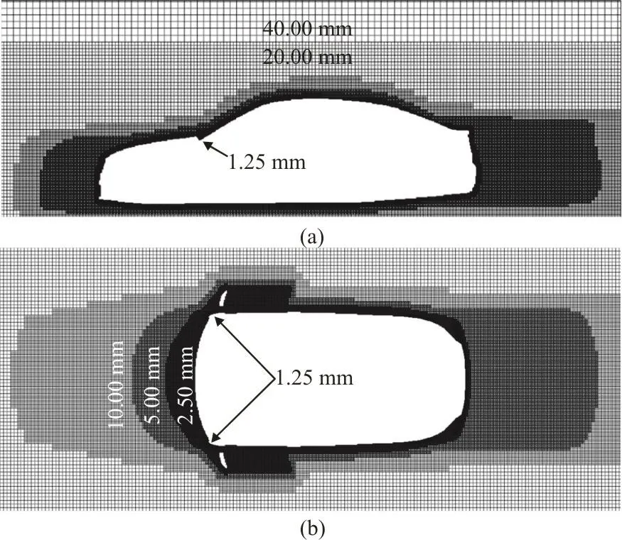
Fig. 4 Computational meshes

1.4 Multiphase simulation setup

Unlike the calculation of the aerodynamic force,the calculation of the water contamination of vehicles requires a subdivision of the computational meshes to capture the raindrop and the water film movements.Moreover, the calculation of the coupling of multiple phases to simulate the full vehicle body usually involves a good amount of the computational resources.The balance between the simulation accuracy and the computational costs is achieved in this work by applying the BSD method[9]. Figure 5 shows the flowchart summarizing the BSD method.

Fig. 5 Flowchart of the BSD method

A subdomain is extracted from the entire domain,including the major components, such as the front windshield, the wiper, the rearview mirror, and the side window, which could affect the side-window contamination (Fig. 6). The subdomain boundaries are divided into three parts. Each part is seeded in the same position as that in the simulation by using the velocity and pressure values derived from the average flow of the full vehicle’s aerodynamic simulation. The outlet boundaries are set as the pressure fields in the free flow direction. The side boundaries are established as the outlet, with the velocity and the pressure. The inlet is specified as the flow into the subdomain where the pressure and the velocity, with a designated turbulence intensity, could originate from a steady state, as determined by the aerodynamic simulation. A rain emitter is positioned at the inlet to provide a rain condition of 17 mm/h and a raindrop density of 1 000 kg/m3. The initial velocity is the same as the vehicle speed. The diameters of the raindrops are in the Gaussian distribution; in the range of 1 mm-3 mm. The motion of the wiper is considered in the simulation. The re-entrainment of the film thickness is set as 0.3 mm.

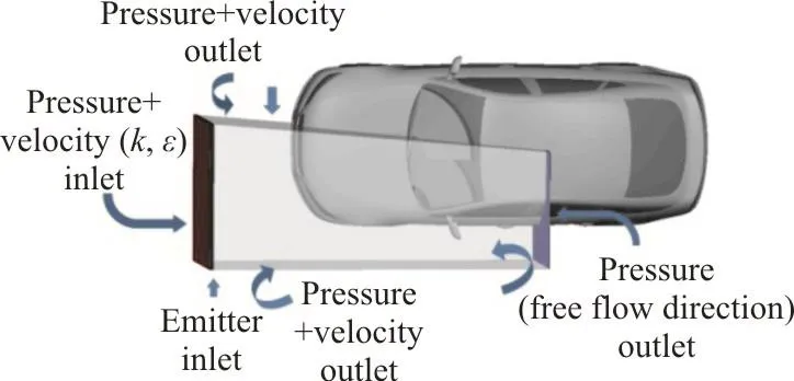
Fig. 6 (Color online) BSD method and boundary condition

1.5 Result validation of the computational fluid dynamics (CFD)

1.5.1 Simulation time independence test

An exact simulation of the external flow field around the vehicle is important not only in determining the accurate aerodynamic drag; but also because it is the first step in the calculation of the water contamination. Furthermore, the movement of a water film is affected by the shear force of the airflow,and the motion trajectories of the raindrops can be tracked from the velocity and the pressure of the flow field. A transient solver is used in this study to capture the flow around the car body, including the separated adhesion and the complex vortex structure. The black curve in Fig. 7 represents the development of the drag coefficient over time, in which it is seen that the values of the drag coefficient vary considerably in the initial stage of the simulation and eventually stabilize around a certain value. The back_avg curve in the same figure represents the mean values over a selected averaging period, with the values being somewhat stable after 6.0×104steps. Subsequently, the drag coefficients are compared with those obtained after four different time steps to avoid the effect of the latter on the numerical simulation. Only a slight difference of Cdvalues between 1.2×105and 1.4×105steps is observed. In view of the computational resource and the efficiency, 1.2×105steps are selected for the calculation of the flow field.

1.5.2 Validation of the numerical method

Fig. 7 (Color online) Cd development over time obtained using a transient solver

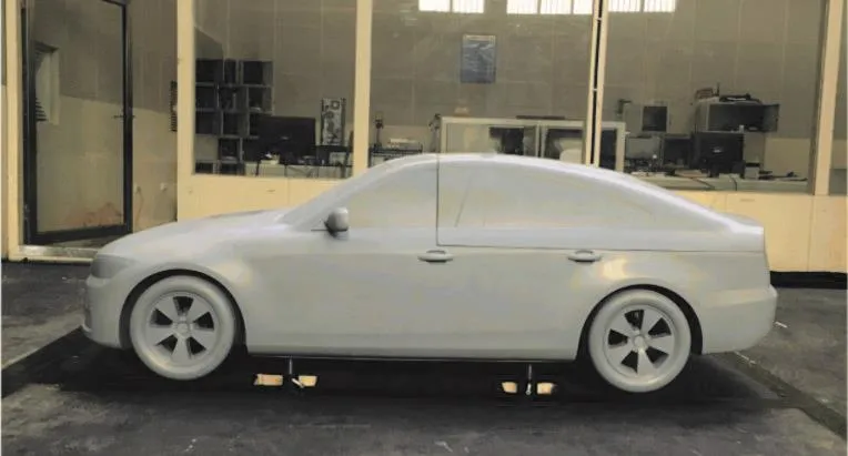
Fig. 8 Wind tunnel and experimental model

Table 1 Comparison of drag coefficients between wind tunnel testing and numerical simulation

A wind tunnel experiment is conducted to verify the simulation results of the CFD. The DrivAer model is built in one-fourth scale and with a smooth chassis.Measurements are made in the return-flow automotive wind tunnel of Jilin University. The dimension of the test section is 4.4 m×2.0 m×8.0 m (Fig. 8). The turbulence intensity of the inflow is less than 0.5%,and the drag is measured by a six-component balance with an accuracy of 0.05%. Table 1 shows a comparison of the drag coefficients between the experimental and numerical simulation results at the same Reynolds number. The relative error between them is 3.9%, indicating that the numerical method can well predict the external flow field of this model.

In fact, the accuracy of the flow characteristics around the vehicle decides how accurate the particles’trajectories are. Jilesen et al.[9]and Hu et al.[17]verified the accuracy of the LBM with the Lagrangian model by experimental results. They comprehensively evaluated the key numerical settings (including the turbulence model, the mesh strategy, the particle model and the film model) for predicting the water contamination on the vehicle. We adopt the optimal numerical settings (the same numerical method and the similar mesh strategy) for simulating the water contamination on the side window as in the above mentioned studies. Therefore, it is appropriate to assume that the present numerical method and simulation settings are suitable for the investigation of the water contamination on the vehicle in this paper.

1.6 Validation of the BSD method

The water volume distribution of the BSD method is compared with that in the full simulation to validate the BSD method’s accuracy. The differences are negligible, at the same time and position, and most of the distributions are consistent with one another(Fig. 9). These differences are caused by the transient simulations and within a reasonable range, which indicates that the water contamination on side windows can be predicted effectively using the BSD method.

The work is carried out on the HPC highperformance computer clusters with 21 nodes,including 19 computing nodes, 1 storage node, and 1 management node, in Jilin University. Each computing node has 12-core processor (2.3 GHz) and 128GB ROM. The calculation time for a full domain simulation is 12 288 CPU hours, while the calculation time for the BSD method is 2 304 CPU hours.Compared with the full domain simulation, the simulation time of the subdomain is reduced by 81.25%, indicating that the simulation efficiency is significantly improved.

2. Optimization process

2.1 Selection of optimal parameters

The cause of the side window contamination of this model should be analyzed before the water management optimization to improve the efficiency of the proposed optimization scheme. Three sources of the water accumulation are analyzed, as mentioned previously. As shown in the film velocity in Fig. 10,the raindrops deposited on the windshield are moved to the A-pillar by the wiper’s periodic action, resulting in a deep water film on the surface of the A-pillar.Meanwhile, as shown in Fig. 11 the skin friction on the surface of the A-pillar is sufficiently large (greater than 2.5 N/m2[17]) to push the water film on the windshield to the side window, which indicates that the rain, which falls on the windshield, will flow over the A-pillar and move to the side window. However,the shearing force on the side window area is small,and the water film moves downward under the action of gravity, impairing the driver’s field of vision.

The water film on the rear mirror surface is gradually thickened with the progress of the calculation time, and the breakup of the water droplets from the edge of the mirror is less constrained under the action of the airflow’s strong shear force. However,as shown by the black circle in Fig. 12, the circular eddy motions of the water droplets, combined with the airflow, do not impair the driver’s main visual field.

As shown in Fig. 13, the airflow separates first and then the air flows along the rear of the side window due to the strong A-pillar vortex, and the raindrops in the incoming stream do not directly affect the front of the side window.

According to the analysis of the side-window contamination of this model, the leading cause of the water contamination on the side windows is clearly the A-pillar overflow, caused by the lateral component of the radial aerodynamic flow and the periodic motion of the wipers. In terms of the A-pillar optimization, numerous optimized parameters can be freely accessed. In this study, only three parameters of the A-pillar section are selected as the design variables, as shown in Fig. 14, Table 2.

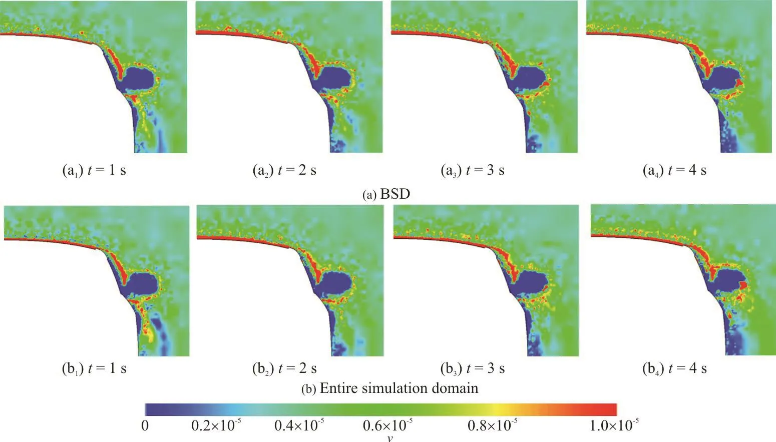
Fig. 9 (Color online) Comparison of water volumes, =1.1m X

Fig. 10 (Color online) Water film velocity

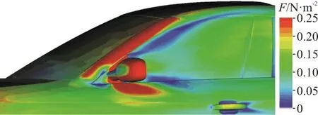
Fig. 11 (Color online) Average skin friction

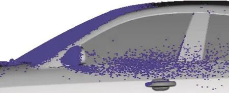
Fig. 13 (Color online) Hitting points

The two reasons for choosing the above parameters are as follows. First, the main purpose of this study is to verify the optimization framework for the side window’s water contamination, which can be best depicted by using relatively few parameters to keep the simulation time within a reasonable range. Second,the size of the car and the impact of the A-pillar modifications on the ergonomics and the aesthetics should be considered.

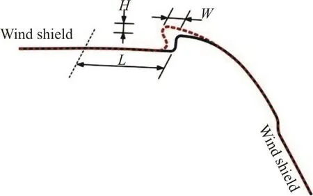
Fig. 14 (Color online) Design variables used for optimization

Table 2 Optimization parameters

2.2 Kriging model method

The Kriging approximation model is known to be an unbiased and optimal estimation method when certain variables in a limited area need to be considered for correlation and variability[21]. The Kriging approximation model combines the global model and the local bias, which can be expressed as

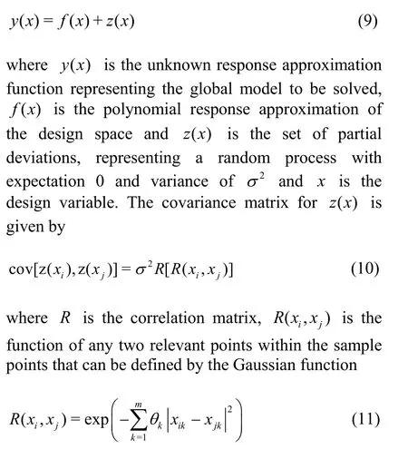
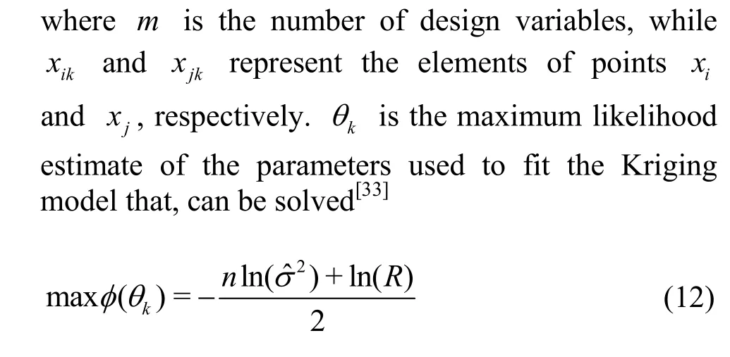
2.3 Design of experiments

where Rsis the number of pixels for the water distribution area of the side window, Rwis the total number of pixels on the side window. Both variables are calculated by using the Photoshop software. S is the area of the side window.

2.4 Modeling for Cd and Sw by using the Kriging model

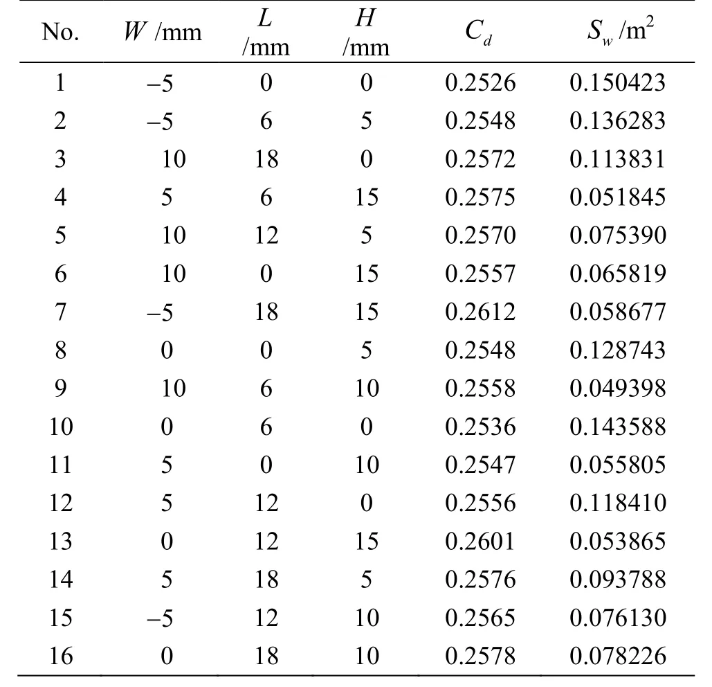
Table 3 Orthogonal table and calculation results of the samples

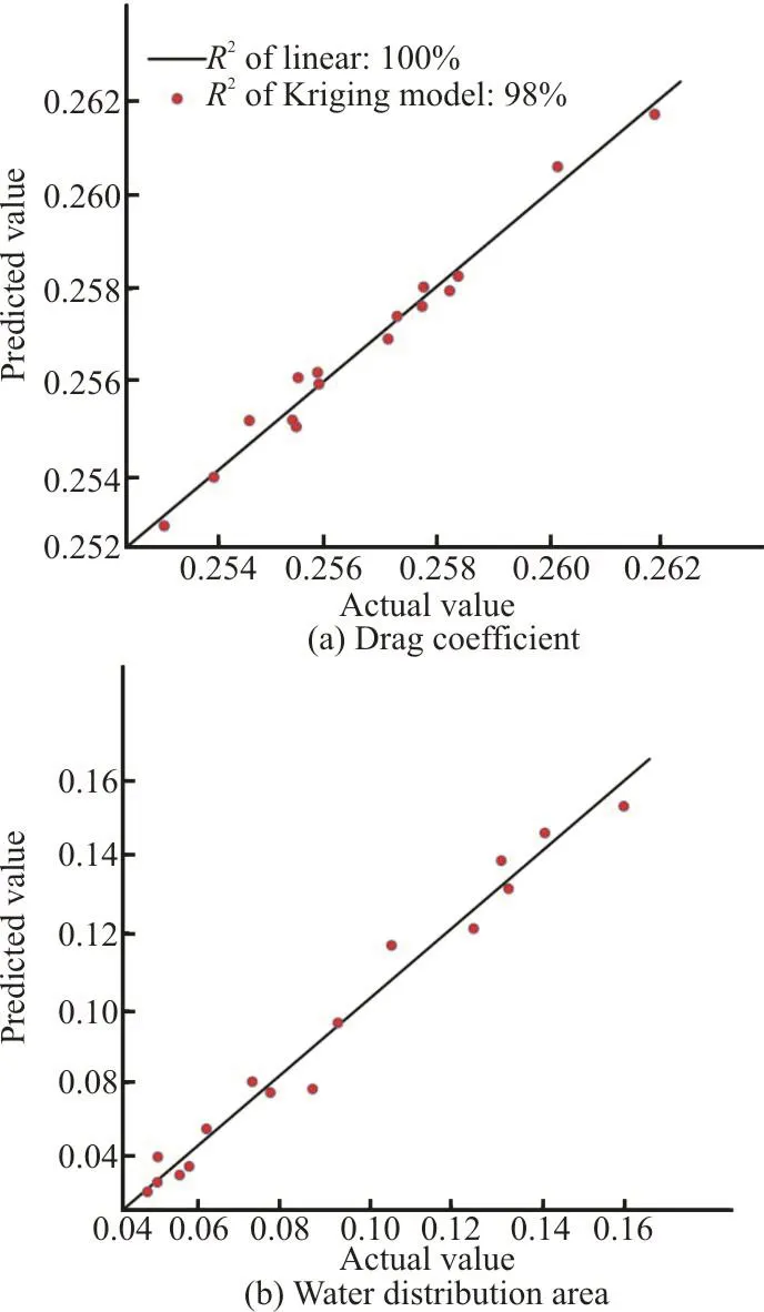
Fig. 15 (Color online) Fitting accuracy of the Kriging model

Table 4 Evaluation coefficients of Kriging model

2.5 Global optimization

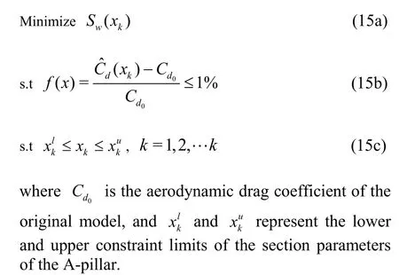
The purpose of this work is determined ways to reduce the water contamination on the side windows,so the water distribution area is the focus of the main optimization objective. At the same time, the changes of the parameters of the A-pillar section may increase the aerodynamic drag, to have a great influence on the fuel economy. Therefore, the impact on the aerodynamic drag should be taken into account in the optimization process for the side-window contamination. To obtain a reasonable combination of the design variables, the multi-objective optimization is carried out with the goal of minimizing the side window(Sw)contamination within a specified range of the Cdvariation. The optimization function can be expressed as follows:

With the approximate model based on the Kriging model, the multi-island genetic algorithm(MIGA) is selected for the global optimization. The MIGA method can be used to select several subpopulations from an original population, make a selection,perform a crossover, and conduct mutation genetic operations on each island while simultaneously but periodically selecting several individuals on each island to be migrated to other islands. The migration between islands allows for the optimal model to be greatly improved during the optimization process[24-25].The optimization results in this work are accurate enough by setting the number of subpopulations to 16,the number of islands to 10, the number of evolution generations to 300, and the total number of evaluations to 48 001. The optimal model is constructed after performing the global optimization along with the settings mentioned above. The corresponding scatterplot is shown in Fig. 16. Then, based on the parameters obtained by the GA method, the original model is deformed into the optimal model, to be used for the CFD simulation. Table 5 shows the error between the GA and CFD calculations, in which the relative error of the aerodynamic drag coefficient is 0.02% and that of the side window soiling area is 2.3%. These results suggest that the optimal model obtained by the MIGA method has a high accuracy and can meet the engineering requirements.

Fig. 16 (Color online) Scatterplot based on Cd and Sw

Table 5 Accuracy of the GA method

3. Results and discussions

Table 6 shows a comparison of the design parameters and the optimization targets between the original and optimized models. After a series of optimizations, the total side-window contamination area is decreased by 66.93%, with the aerodynamic drag being increased only slightly (0.41%). Compared with the values in the original model, the height of the A-pillar section in the optimized model is increased by 11.22 mm, the length is extended by 1.27 mm, and the width is broadened by 7.77 mm (Fig. 17).

Table 6 Design variables and optimization results between the original and optimal models.

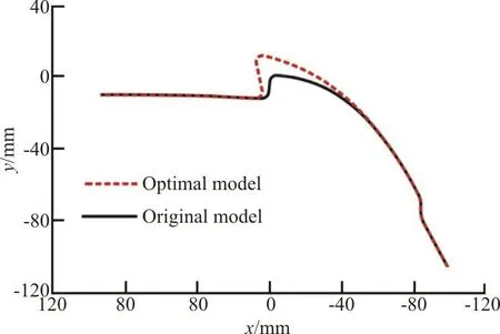
Fig. 17 (Color online) Comparison between original and optimal model

The water film thicknesses at the four representative measured points of the original and optimization models are shown in Fig. 18. The water film thickness at each point on the side window is lower than that of the original model during the whole simulation time,especially at points 1, 2 and 3. The water film on the windscreen flows to the A-pillar under the action of the wiper. For the original model, the water film thickness at point 1 is thus increased rapidly to 0.03 mm within 0.5 s. The water film thickness is fluctuated slightly under the influence of the wiper’s periodic motion. After optimizing the section parameters of the A-pillar, the main view of the side window becomes clear (Fig. 19(b)). However,although the A-pillar’s overflow is effectively reduced through the optimization, drops still fall from the edge of the A-pillar through the action of the vortex, and the incoming flow falls at point 1 in the optimal model,making the water film to rise slowly. Owing to the influence of the gravity, the water film thickness at point 4 becomes balanced within a shorter time than at point 1, and the thickness becomes stable within approximately 0.045 mm (Fig. 18(b)). The water film in the original model overflows from the A-pillar to the side window and reaches the point 3 in 2 s. The water film thickness is increased rapidly to 0.045 mm in a short time and then becomes stable. As shown in Figs. 18(c), 19, the point 3 of the optimal model is not affected by the A-pillar overflow, and the rain droplets of the incoming flow and the vortex on the rear mirror are deposited on this region, increasing slowly the water film thickness, but without impairing the driver’s main view. Changing the parameters of the A-pillar surface also alters their effects on the A-pillar and mirror vortex. The corresponding differences between the original and optimized models at point 4 are shown in Fig. 18(d).

Fig. 18 (Color online) Water film thicknesses of the measured points on the side window regions of the original and optimal models

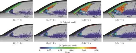
Fig. 19 (Color online) Comparison of water film thicknesses between the original and optimized models

Figure 19 shows that the water contamination area on the side window of the original model is much larger than that of the optimized model. It can be seen that the water film on the windscreen of the original model easily breaches the A-pillar and flows to the side glass, obscures the vision of the drivers. However,with the optimized model, the water is pushed towards the A-pillar when the wipers are active, to form a single rivulet, moving into the roof instead of going down to the side window. Therefore, while the contamination area of the original model increases with the time, that of the optimized model maintains a clear region.

The difference between the water phase distributions on the side windows of the original and optimized models is illustrated in terms of the water film velocity and the shear stress (Figs. 20, 21). Under the action of the wiper, the water on the windshield flows towards the edge where the front windshield meets the A-pillar. Subsequently, the water is driven towards the A-pillar surface by the horizontal velocity(Fig. 20(a)). The surface shear force is one of the main driving forces of the film motion. When the shear force is larger than 2.5 N/m2, the water film tends to move with the near-wall airflow[26]. In this work, the presence of a streamline on the A-pillar surface (Fig.21(a)) indicates that the skin friction of the A-pillar surface is consistent with the horizontal velocity of the water film. This finding further suggests that the water can be pushed towards the side window under the influence of the water motion. Furthermore, a visible region of low shear stress could be observed on the side window where the water from the A-pillar flows downward to the area of the driver’s field of vision due to the influence of gravity. Unlike the shear stress direction in the A-pillar surface in the original model,that in the optimized model is opposite to the water film velocity, a phenomenon that enables the water to gather on the A-pillar surface. As shown in Fig. 20(b),the water film at the edge of the A-pillar in the optimized model is thicker than that in the original model. The streamline on the top of the A-pillar in Fig.21(b) indicates that the shear force can act in other directions than that of gravity. This phenomenon further suggests that the water, which tends to flow downward due to gravity, can be pushed back to the top of a vehicle, and a driver’s view is hardly impaired.

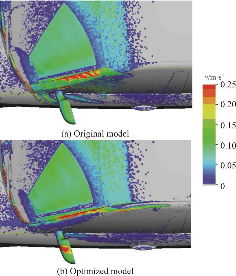
Fig. 20 (Color online) Comparison of water film velocities

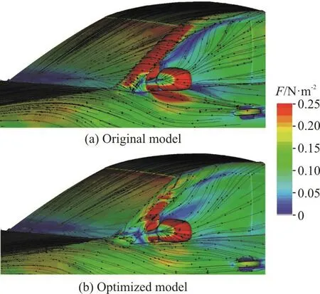
Fig. 21 (Color online) Comparison of surface shear stress between the original and optimized models

4. Conclusions

This study presents a feasible and efficient simulation method and optimization framework for the design of the A-pillar section parameters to reduce the water contamination on the side window of vehicles within the permissible range of the aerodynamic drag.The following conclusions are obtained from this study:

(1) The flow fields in the optimal and original models are analyzed. The shear force direction on the A-pillar surface is opposite to that of the water film movement in the optimized model. This phenomenon prevents the water film from overflowing to the side window.

(2) The water contamination area in the optimal model is reduced by 66.93%, while the aerodynamic drag is increased only by 0.41%, as compared to those in the original model. These findings indicate that the parameters used for the A-pillar section, obtained by using the abovementioned design method, are feasible and effective.

(3) The Kriging model enjoys an excellent fitting accuracy, with both the evaluation coefficients2(R)of Cdand Swexceeding 0.95, by using only 16 sample points. This result indicates the suitability of the optimization design with a long calculation time for a single case, such as the exterior water management of vehicles.

(4) The calculation time of the BSD method is only 18.23% of the entire domain calculation time for a single sample.

(5) The analytical results of the three sources of the water accumulation indicate that the A-pillar’s overflow is the primary source of the water contamination on the side windows of the DrivAer model. This work provides a new direction of reducing the water contamination on the side window of vehicles and might be applied in the engineering practice.

Acknowledgement

This work was supported by the Graduate Innovation Fund of Jilin University (Grant No.419100200651).