Prediction of Logistics Demand via Least Square Method and Multi-Layer Perceptron
WEILeqin,ZHANGAnguo
1 School of Humanities and Teachers’ Education, Wuyi University,Wuyishan 354300, China 2 College of Physics and Information Engineering, Fuzhou University, Fuzhou 350108, China
Abstract: To implement the prediction of the logistics demand capacity of a certain region, a comprehensive index system is constructed, which is composed of freight volume and other eight relevant economic indices, such as gross domestic product (GDP), consumer price index (CPI), total import and export volume, port’s cargo throughput, total retail sales of consumer goods, total fixed asset investment, highway mileage, and resident population, to form the foundation for the model calculation. Based on the least square method (LSM) to fit the parameters, the study obtains an accurate mathematical model and predicts the changes of each index in the next five years. Using artificial intelligence software, the research establishes the logistics demand model of multi-layer perceptron (MLP) neural network, makes an empirical analysis on the logistics demand of Quanzhou City, and predicts its logistics demand in the next five years, which provides some references for formulating logistics planning and development strategy.
Key words: logistics demand; least square method (LSM); multi-layer perceptron (MLP); prediction; strategic planning
Introduction
In recent years, the research on the choice of logistics demand prediction methods can be divided into two aspects: one is based on statistics, such as multiple linear regression prediction, grey theory model, input-output model, Markov chain and other traditional logistics demand prediction methods; the other is the intelligent prediction methods based on intelligent control theory, information and computer science and technology, which mainly include neural networks, support vector machines (SVM) and related improved algorithms.
In the application of traditional statistics based logistics demand prediction method, Wangetal.[1]combined principal component regression and GM(1, 1) prediction model with traditional statistics based logistics demand prediction method to predict the logistics demand of Nanping City from the years 2018 to 2022. By using the combination model of grey chain and Markov chain, Zhang and Li[2]improved the prediction accuracy, quantitatively predicted the cold chain logistics demand of agricultural products in Beijing-Tianjin-Hebei region, and put forward corresponding suggestions and countermeasures, which broke through the limitation of the traditional single model prediction accuracy. Ranetal.[3]used GM (1, 1) of fuzzy prediction to predict the development of freight volume and GDP in Yunnan Province. Gaoetal.[4]constructed a principal component regression model and conducted an empirical analysis on the development of Tai’an City logistics industry based on the selection of development index for the logistics industry, so as to provide reference for the development prediction of the logistics industry. Bietal.[5]constructed a ranking index model to optimize the quantitative index of logistics demand based on grey relational analysis and correlation coefficient analysis for Luzhou City, and constructed the principal component regression model based on the optimized quantitative index of logistics demand and the influencing indices to carry out the model accuracy test. Yuetal.[6]used the index smoothing method to predict the logistics data of Yunnan Province from the years 2009 to 2017. The results showed that the index smoothing method was a short-term prediction method, which was more practical than the multiple linear regression model, grey prediction method and weighted arithmetic average method.
In the application of logistics demand intelligent prediction method based on intelligent control theory, information technology and computer science technology, Zhang and Wang[7]used GM(1, 1)-multi-layer perceptron (MLP) neural network combination model to predict the total logistics volume of China in the future. The results showed that the average prediction error of the combination model was much lower than that of GM(1,1) alone, and the accuracy was greatly improved. Luo[8]used data mining technology for data preprocessing and MLP neural network training technology for data analysis. The results showed little difference from the actual data, so the model and processing model method were effective and feasible. Gao[9]analyzed the main factors affecting the logistics demand of Hainan Province, selected the corresponding economic indicators as the relevant impact indicators of logistics demand prediction, and used the BP neural network model to select the relevant statistical data of Hainan Province from the years 2003 to 2016 to predict the logistics demand of Hainan Province from the years 2017 to 2022. Caoetal.[10]used genetic algorithm to optimize SVM, auto-regressive integrated moving average(ARIMA) and grey prediction method, selected the freight volume data of Guangxi Province from the years 1990 to 2015, and established the logistics demand prediction model. The results showed that the method of genetic algorithm to optimize SVM had better prediction effect. Xiaoetal.[11]took air passenger volume as logistics demand index, established an air passenger volume prediction model based on adaptive network fuzzy reasoning system, and used improved particle swarm optimization (IPSO) algorithm to predict short-term air passenger volume, so as to solve the problem of air transport demand prediction. In order to reduce inventory cost, Jaipuria and Mahapatra[12]collected logistics data of three different manufacturing firms, and used an integrated approach of discrete wavelet transforms (DWT) analysis and artificial neural network (ANN) denoted as DWT-ANN for logistics demand forecasting, and the study indicated the model had good prediction accuracy.
Logistics demand prediction is a complex process. Traditional prediction methods and intelligent prediction methods have their own advantages and disadvantages. In order to achieve the ideal prediction effect, the choice of scientific and reasonable logistics demand prediction method is the key to achieve accurate logistics demand prediction[13-14]. From the perspective of index selection and prediction method selection, this paper draws on the advantages of traditional prediction methods and intelligent prediction methods, and creatively adopts least square method-MLP (LSM-MLP) combination model to predict the logistics demand of Quanzhou City in the next five years.
1 Index System Construction
1.1 Data collection
Logistics demand is the derivative demand of national economy, including the type and quantity of materials flowing in space and time. Since these contents are quantifiable, they are also collectively referred to as logistics requirements. People usually use the total amount of social logistics transportation, inventory processing, distribution, individual indirect logistics or total output value of social logistics in a particular region to express the regional logistics demand, but the statistical scope of China’s logistics demand has not been unified. Existing historical data do not directly reflect current logistics needs and composition[15-20]. Previous researches indicated that available logistics demand measurable index and highly correlative influencing indexes should be selected reasonably[1, 21-23]. Considering the availability and statistical consistency of the data, this paper proposes that it is feasible to take freight volumeYas the research object. Eight other indicators, including gross domestic product (GDP)X1, consumer price index (CPI)X2, total import and export volumeX3, port’s cargo throughputX4, total retail sales of consumer goodsX5, total fixed asset investmentX6, highway mileageX7, and resident populationX8, were selected as the influencing factors of freight volume in Quanzhou City (shown in Fig. 1).
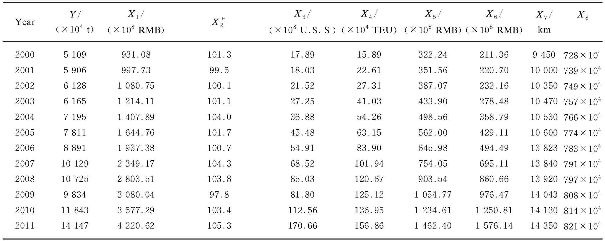
Table 1 Statistical data of economic indicators related to logistics demand scale of Quanzhou City from the years 2000 to 2019

(Table 1 continued)
1.2 Methodologies
The eight independent variables are modeled independently, and the LSM is used to fit the parameters, and the fitting variance is recorded. LSM is characterized by clear principle, simple algorithm, fast convergence speed, easy to understand and master, and has been widely used in parameter estimation. After the accurate mathematical model is obtained, eight changes of each index in the next five years are predicted.
Then, according to the incremental changes of the eight indicators year by year, MLP artificial neural network is constructed by artificial intelligence software MATLAB 2020a to study the incremental changes, so as to obtain the development trend of freight volume in the next five years, as shown in Fig. 1.

Fig. 1 Five-year prediction method
2 Data Analyses and Prediction
2.1 Mathematical modeling for the eight external indicators
The relative definitions are described as follows[24].
The sum of squares due to error (SSE): this statistic measures the deviation of the fitting value of the response. The closer a value is to 0, the better match it is.
Coefficient of determination (R2): this statistic measures how successful the fit is in explaining the variation of the data. The value is between 0 and 1, and a value closer to 1 indicates a better fit.
Coefficient of freedom adjustment determination (adjustedR2): the closer the value is to 1, the better the match is. When additional coefficients are added to the model, it is usually the best indicator of quality.
2.2 Model for GDP
The fitting result of GDP is (95% confidence interval)fG(x)=17.89x2+60.98x+743.3 (shown in Fig. 2), wherex=1, 2, …,n, which represents the serial number of the special year from 2000, the same to those in Figs. 3-9.
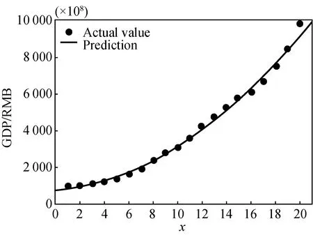
Fig. 2 Model fitting of 20-year data of GDP with abscissa representing years starting from 2000
The matching degree is as follows: SSE is 4.346×10⁵,R2is 0.996 9, and adjustedR2is 0.996 6 respectively.
2.3 Model for CPI
The fitting result of CPI is (95% confidence interval)fC(x)=0.000 9035x4-0.0370 2x3+0.460 8x2-1.617x+102 (shown in Fig. 3).
The matching degree is as follows: SSE is 33.63,R2is 0.417 5, and adjustedR2is 0.262 2 respectively.
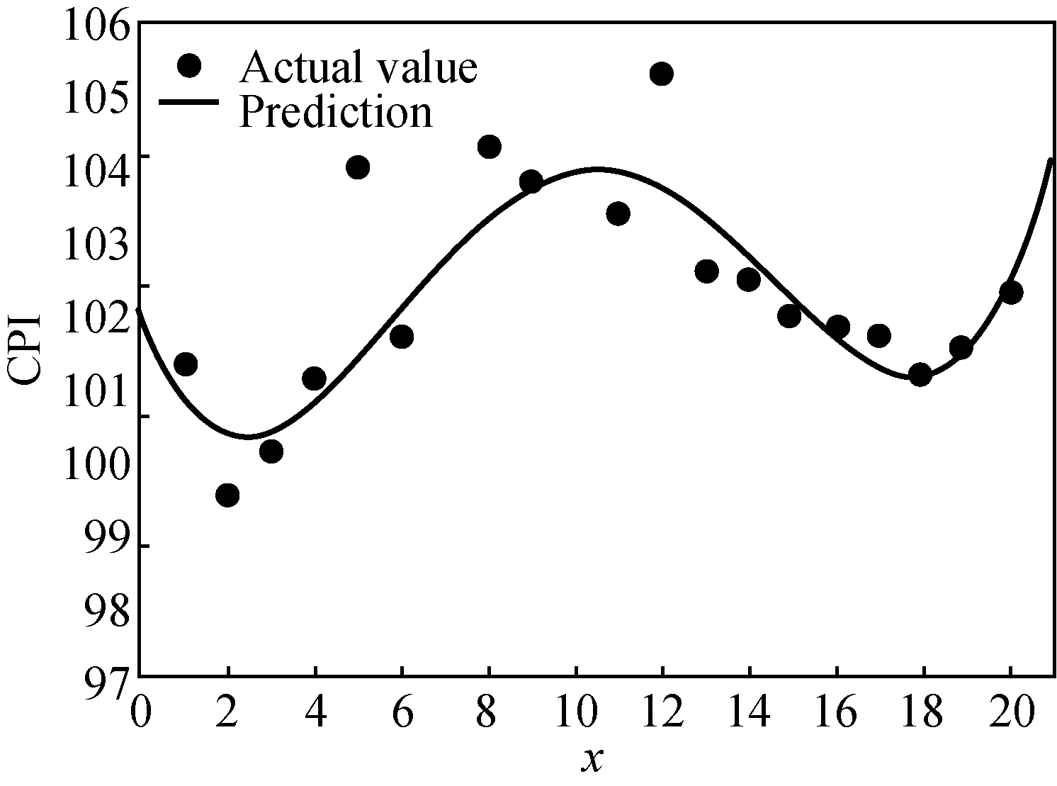
Fig. 3 Model fitting of 20-year data of CPI with abscissa representing years starting from 2000
2.4 Model for total import and export volume
In Fig. 4 the fitting result of total import and export volume is (95% confidence interval)fI(x)=2 722 sin(0.007 335x-0.024 51)+48.91sin(0.558 7x+0.020 11)+31.09 sin(0.933 6x+0.890 6).
The matching degree is as follows: SSE is 1 485,R2is 0.993 7, and adjustedR2is 0.989 1 respectively.
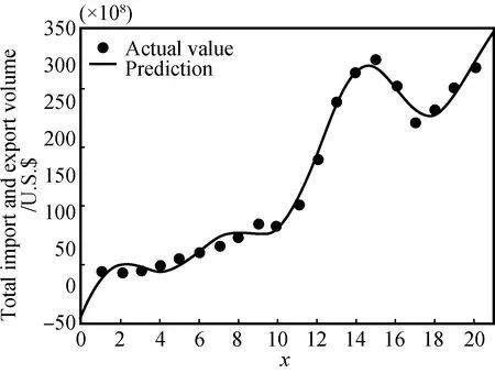
Fig. 4 Model fitting of 20-year data of total import and export volume with abscissa representing years starting from 2000
2.5 Model for port’s cargo throughput
In Fig. 5 the fitting result of port’s cargo throughput is (95% confidence interval)fP(x)=451.2sin(0.102 3x+0.259)+350.6sin(0.144 9x+3.298)+47.09sin(0.291 8x+5.022).
The matching degree is as follows: SSE is 194,R2is 0.998 3, and adjustedR2is 0.997 respectively.
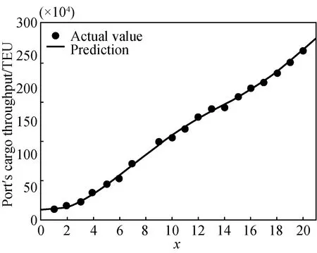
Fig. 5 Model fitting of 20-year data of port’s cargo throughput with abscissa representing years starting from 2000
2.6 Model for total retail sales of consumer goods
The fitting result of the total retail sales of consumer goods is (95% confidence interval)fT(x)=9.814x2-26.61x+363.1 (shown in Fig. 6).
The matching degree is as follows: SSE is 878 6,R2is 0.999 6, and adjustedR2is 0.999 6 respectively.
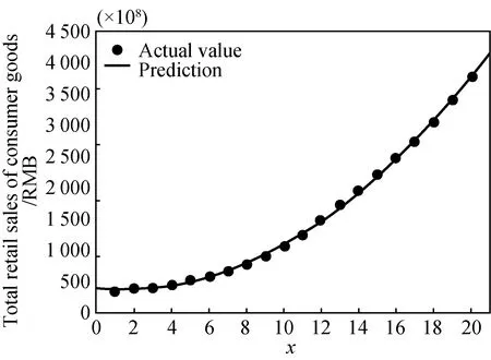
Fig. 6 Model fitting of 20-year data of total retail sales of consumer goods with abscissa representing years starting from 2000
2.7 Model for total fixed asset investment
The fitting result of the total fixed asset investment is (95% confidence interval)fF(x)=-0.108 2x4+4.219x3-35.88x2+142.2x+66.92 (shown in Fig. 7).
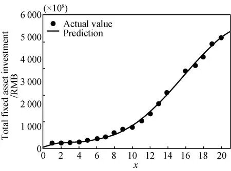
Fig. 7 Model fitting of 20-year data of total fixed asset investment with abscissa representing years starting from 2000
The matching degree is as follows: SSE is 8.364×10⁴,R2is 0.998 4, and adjustedR2is 0.997 9 respectively.
2.8 Model for highway mileage
The fitting result of highway mileage is (95% confidence interval)fH(x)=-0.863 8x3+22.62x2+339.1x+904 8 (shown in Fig. 8).
The matching degree is as follows: SSE is 7.184×10⁶,R2is 0.954 2, and adjustedR2is 0.945 7 respectively.
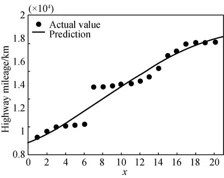
Fig. 8 Model fitting of 20-year data of highway mileage with abscissa representing years starting from 2000
2.9 Model for resident population
The fitting result of resident population is (95% confidence interval)fR(x)=-0.079 44x2+9.405x+720.5(shown in Fig. 9).
The matching degree is as follows: SSE is 18.12,R2is 0.999 5,and adjustedR2is 0.999 5 respectively.
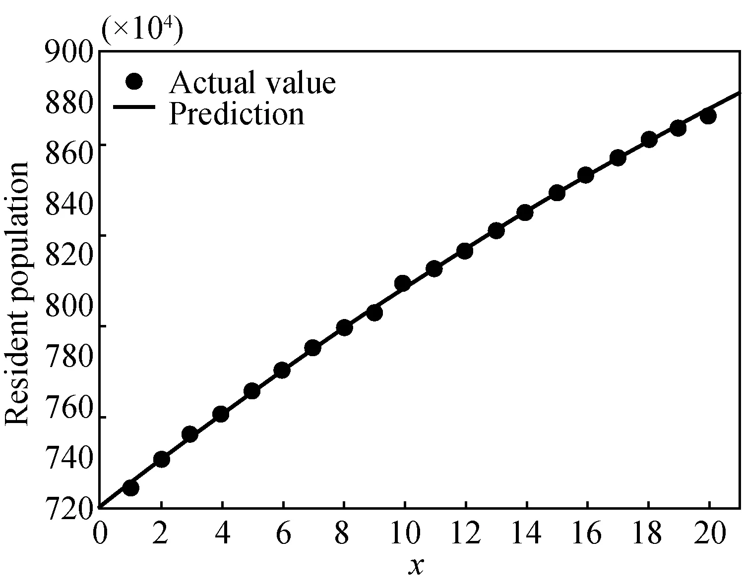
Fig. 9 Model fitting of 20-year data of resident population with abscissa representing years starting from 2000
3 Multivariate Prediction Based onExternal Indicators
Based on the mathematical modeling of eight external indicators in section 2, we can independently predict the respective values of the eight indicators in the next five years, as shown in Table 2.

Table 2 Respective values of the eight indicators in the next five years
The increment of each indicator is predicted by MLP neural network. The 8-H-1 network structure is used,i.e., 8 refers to input nodes, H refers to hidden nodes and 1 refers to output node. The structure of a single MLP is shown in Fig. 10. Due to the small amount of data, we adopt the idea of integrated study to ensure the stability of model output. As shown in Fig. 11, we build a model composed of five MLP units, among which the number of hidden layer nodes of the five MLP units is 4, 6, 8, 10, and 12 respectively.
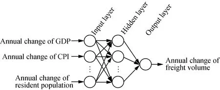
Fig. 10 Structure of MLP neural network prediction model
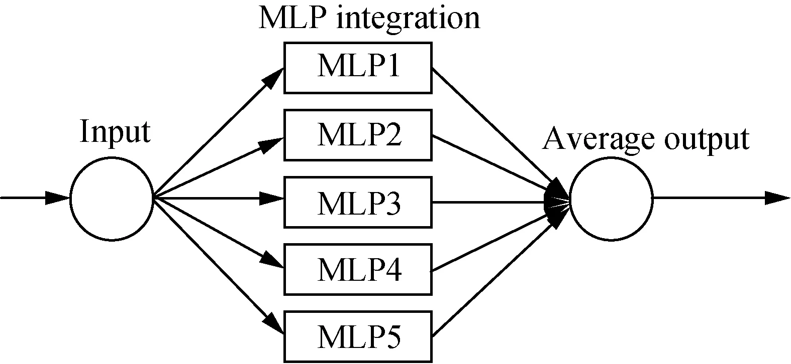
Fig. 11 Prediction model consisting of five MLP units
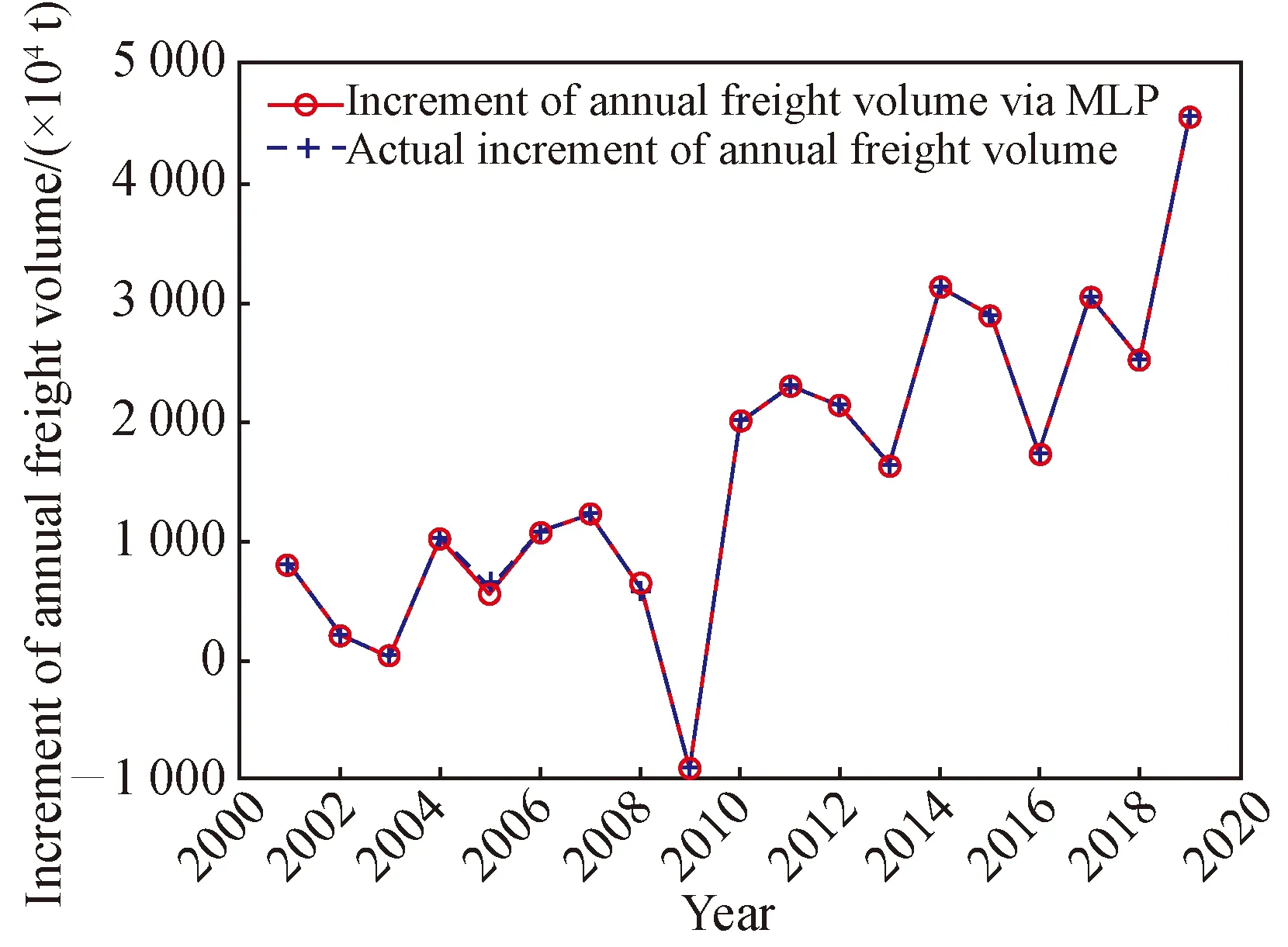
Fig. 12 MLP network fitting error effect after training
Figure 12 shows the error of one MLP network after training based on the data from the years 2000 to 2019. As can be seen from Fig. 12, the network can well fit the annual increment of total freight volume over the past 20 years. We use a well-trained MLP network to predict the annual growth rate of freight over the next five years. The predicted outputs of the five MLP units we trained over the next five years are shown in Table 3.

Table 3 Predicted values and comprehensive average values of five MLP units
Therefore, the predictive values of total freight volume from the years 2020 to 2024 are respectively shown in Table 4.
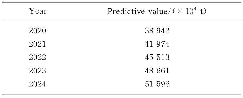
Table 4 Predictive values of total freight volume in Quanzhou City
4 Practical Implications and Theoretical Contributions
From the overall trend, Quanzhou logistics demand is on the rise. Total freight volume will exceed 400 million tons in 2021 and over 500 million tons in 2024. In theory, the accurate prediction of Quanzhou logistics demand can provide important basis for the formulation of logistics development strategic planning, logistics infrastructure scale and logistics management scheme, and provide concrete and reliable quantitative support for the development of logistics industry. In practice, accurate prediction of logistics demand for Quanzhou City is helpful for government departments to reasonably plan and control the development scale and speed of logistics industry, which is of practical significance to develop regional economy and reduce waste[25-27]. Regional logistics demand prediction is to find the internal relationship between regional economy and regional logistics and provide necessary decision-making data and basis for regional logistics planning[28-31]. These forecasting data are collected in the relatively ideal economic environment, excluding the impact of black swan or grey rhino incidents such as COVID-19.
5 Conclusions
There is a strong correlation between the logistics demand and the relevant index of regional economic development. The development of regional logistics industry can not be separated from its economic development level, which should be highly coordinated with regional economic development to avoid the phenomenon of insufficient or excessive investment in logistics infrastructure construction and insufficient or excessive logistics supply capacity. Based on the study of the internal relationship between regional economy and logistics demand, this paper proposes a logistics prediction model based on LSM-MLP neural network, and reveals the internal nonlinear mapping relationship between regional economy and regional logistics demand. At the same time, it forecasts the logistics demand of Quanzhou City in the next five years through empirical research, which proves that the model has high prediction accuracy and validity. Therefore, it provides a new idea and method for regional logistics demand prediction, which is of certain theoretical and practical significance, especially for Quanzhou City that is defined as the Pilot Zone of the 21st-Century Maritime Silk Road. The factors influencing the regional logistics of coastal cities include not only intra-regional factors, but also extraterritorial factors such as inter regional competition pressure, hinterland economic expansion brought by transportation improvement, and thus the issue will be further discussed in future research.
 Journal of Donghua University(English Edition)2020年6期
- Journal of Donghua University(English Edition)的其它文章
- Effect of Different Types of Structural Configuration on Air Distribution in a Compact Purification Device
- Measurement of International Competitiveness of Clothing Industry under the Background of Value Chain Reconstruction
- Counterexample of Local Fractional Order Chain Rule and Modified Definition of Local Fractional Order
- Deep Knowledge Tracing Embedding Neural Network for Individualized Learning
- Design and Application of Coordinator App Based on Needs Survey
- Optimization Method of Bearing Support Positions in a High-Speed Flexible Rotor System
