
The impacts of modeling global CO2 concentrations with GEOS-Chem using different ocean carbon fluxes
2019-12-03 07:53:12ZHANGShanandTIANXiangjun
ZHANG Shan and TIAN Xiangjun
aInternational Center for Climate and Environment Sciences,Institute of Atmospheric Physics,Chinese Academy of Sciences,Beijing,China;
bCollege of Earth and Planetary Sciences, University of Chinese Academy of Sciences, Beijing, China; cCollaborative Innovation Center on Forecast and Evaluation of Meteorological Disasters, Nanjing University of Information Science and Technology, Nanjing, China
ABSTRACT The rise in atmospheric carbon dioxide (CO2) concentrations caused by human activities is leading to global climate change, which poses a threat to human development and survival. This study analyzed the distribution of the ocean carbon flux with interannual changes and compared it with the climatological ocean carbon flux to deepen our understanding of carbon sources and sinks. To simulate global CO2 concentrations for the years 2008-2010, the ocean carbon flux with interannual changes and the climatological ocean carbon flux were used to drive the GEOS-Chem model, an atmospheric chemical transport model. The simulated values were compared with the CO2 concentrations at nine observation stations to explore the influence of interannual changes in the ocean carbon fluxes on the simulated CO2 concentrations. The authors found that the difference between the two simulation results was greater in the Southern Hemisphere all year, and the difference in autumn was the largest. Compared with the observations, the simulated CO2 concentration of the ocean carbon flux with interannual changes is closer to the observations,indicating that this simulation is more accurate.
KEYWORDS Carbon sources and sinks;CO2 concentration; GEOSChem model; Ocean carbon fluxes
1. Introduction
Atmospheric carbon dioxide (CO2) is an important greenhouse gas that is principally responsible for the anthropogenic impact on the Earth's energy balance in the process of global warming (Knohl and Veldkamp 2011). The rate of change in the atmospheric CO2concentration depends not only on human activities but also on biogeochemical and climatic processes and their interactions with the carbon cycle (Falkowski et al. 2000). CO2in the ocean is a key control link of the global carbon cycle and plays a major role in the carbon flow among the atmosphere, lithosphere, hydrosphere,and biosphere. The exchange of heat and energy between the ocean and atmosphere has an important effect on climate change.
The distribution of CO2in the ocean varies greatly,and is affected by physical, chemical, and biological factors. Consequently, the quantitative estimation of the carbon absorption, transfer, and burial rates in the ocean has become an important part of marine science(Zhang, Wang, and Chen 2000; Shi et al. 2014). It is estimated that the ocean offsets 30%-50% of anthropogenic CO2, which equals an annual mean uptake of~2 Gt C yr-1, and the oceanic CO2uptake is estimated using ocean-atmosphere carbon-cycle models(Siegenthaler and Sarmiento 1993). In principle, direct measurements of the atmosphere can be used to estimate the net flux across the interface between the ocean and atmosphere, which is known as micrometeorology, but this is difficult to do in practice because of the slow rate of CO2exchange (Xu et al. 2004).Broecker et al. (1986) measured the global average CO2exchange rate using a radioisotope method.Gruber and Keeling (2001) evaluated the isotopic airsea disequilibrium of CO2based on the reduced isotopic ratio (δ13C) of dissolved inorganic carbon.Takahashi et al. (2009) reported the global net sea-air CO2ocean fluxes based on 3 million measurements of surface water partial pressure of CO2(pCO2) in the reference year 2000 and obtained a value of -1.42 Pg C yr-1.
Considering the absorption of CO2by the ocean, we first analyzed the seasonal variation and spatial distribution of ocean carbon fluxes. Since the annual global ocean sink is gradually increasing, we ran GEOS-Chem driven using two ocean carbon fluxes to examine the importance of interannual variation in the ocean carbon flux to simulate the CO2concentration.
2. Model and data
2.1 Model and experimental design
GEOS-Chem is a global three-dimensional model of atmospheric chemistry driven by meteorological inputs from the Goddard Earth Observing System (GEOS) of the NASA Global Modeling and Assimilation Office.GEOS-Chem can perform many different chemical simulations, such as tropospheric ozone-NOx-hydrocarbon chemistry (Bey et al. 2001). Using GEOS-Chem et al. (2004) simulated the CO2concentration in Asia.Nassar et al. (2010) modified the CO2emissions from shipping, aviation, fossil fuel burning, terrestrial biospheric exchange, biomass burning, and ocean exchange.
In this study, we used the GEOS-Chem ver. v11-01 driven by the MERRA-2 meteorology fields to simulate global atmospheric CO2with a horizontal resolution of 2° latitude × 2.5° longitude and 72 vertical levels.
2.2 Ocean flux data and atmospheric CO2 observations
The Carbon Dioxide Research Group at the Lamont-Doherty Earth Observatory (LDEO) has produced a climatology of monthly CO2sea-air fluxes based on 3 million measurements of pCO2in ocean water. They estimated the net sea-air CO2flux (F) using:

where κ is the CO2gas transfer velocity, α is the solubility of CO2in the ocean, and ΔpCO2is the sea-air pCO2difference in the 2000 reference (Takahashi et al.2009).
The climatological data estimated by Takahashi et al.(2009) have been used in GEOS-Chem (Nassar et al.2010). Since the annual global ocean sink is gradually increasing, Takahashi et al. (2009) also assumed a trendof 1.5 μatm yr-1for ocean pCO2by combining this with the GLOBALVIEW-CO2. Table 1 shows the global annual sea-air fluxes with scaling for 2000-2013 (data from Nassar et al. (2010)).
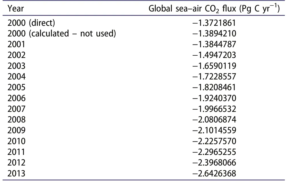
Table 1. Interannual variation in the global annual sea-air fluxes after applying scaling at 1.5 μatm yr-1.
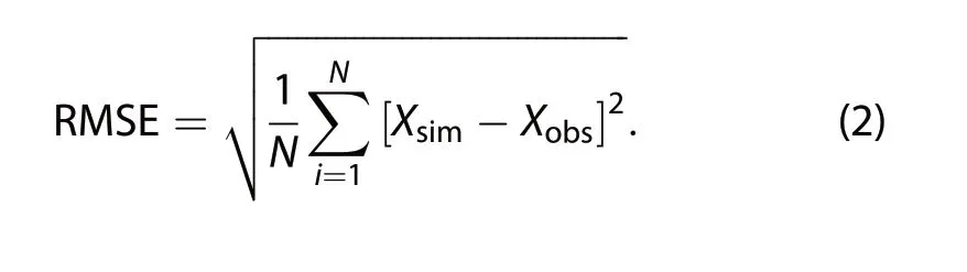
We used observation data for nine months from the National Oceanic and Atmospheric Administration(NOAA)Earth System Research Laboratory(ESRL)surface flask sampling data as the reference for the simulation.The root-mean-square error(RMSE)was used to evaluate the deviation between the CO2concentration simulated using different ocean carbon fluxes and ground observation data. The smaller the value was, the closer the simulated value was to the observed value:
3. Results
3.1 Global distribution and seasonal variation of the ocean fluxes
Figure 1 shows the spatial distribution of the ocean carbon fluxes in different seasons. The equatorial Pacific Ocean, especially in the eastern Pacific, had weak seasonal variation and always showed a wide range of carbon sources. The carbon source located along the equatorial Atlantic Ocean tended to shrink in summer, while the release of CO2in the northwest Indian Ocean was significantly enhanced in summer (Figure 1(e,h)), which is related to the upwelling of CO2caused by the Indian summer monsoon (Goyet, Millero, and O'Sullivan et al.1998). In the mid-latitudes of the Northern Hemisphere, the Atlantic, Indian, and Pacific Oceans had weak CO2air-sea fluxes in summer, but were strong carbon sinks in winter (Figure 1(a,b)). This is due to the winter cooling of waters transported poleward (Takahashi et al. 2009). Mid-latitude regions of the Southern Hemisphere served as sinks in all seasons; however, there was a band of carbon sources around 60°S and 60°N in the summer and fall. CO2release came mainly from a large amount of ice water along the coast of Antarctica, and the slowly moving ice water greatly altered the sea-air CO2flux.
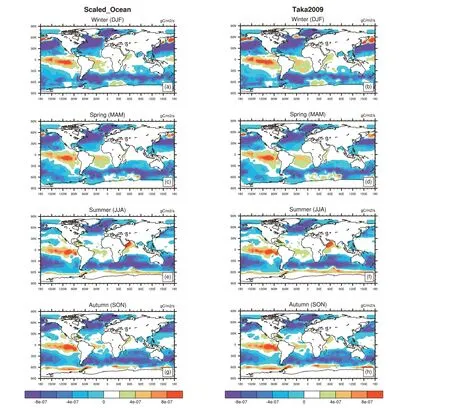
Figure 1. Spatial distribution of the scaled ocean and taka ocean fluxes in different seasons. The scaled ocean is the annual mean value for 2008-2010.
Comparing the global spatial distribution of carbon fluxes of the two oceans, the carbon sources of the interannual ocean carbon flux called the Scaled Ocean over the tropical Atlantic were relatively weak, especially in summer and autumn (Figure 1(e,g)). Similarly, this flux was a significantly weaker carbon source, even taking up CO2around 60°S in autumn and 60°N in spring. However, the climatological ocean carbon flux called Taka2009 absorbed relatively little CO2in the middle and high latitudes of the Northern and Southern Hemispheres.
Figure 2 depicts the variation in the two kinds of ocean carbon flux with latitude. It is more intuitive to determine the change in the ocean carbon source and sink at different latitudes.There were two great absorption centers near 45°S and 40°N. However, the equator consistently released CO2into the atmosphere. In addition, south of 40°S and at 40°N to 60°N, the optimized ocean flux resulted in more net absorption of CO2,while the net exchange was smaller at other latitudes.The Scaled Ocean carbon flux also showed a significant increase with time at mid-latitudes. This ocean flux better reflects the gradual increase in the atmospheric CO2concentration; however, we need to know the ability of the ocean to regulate CO2.
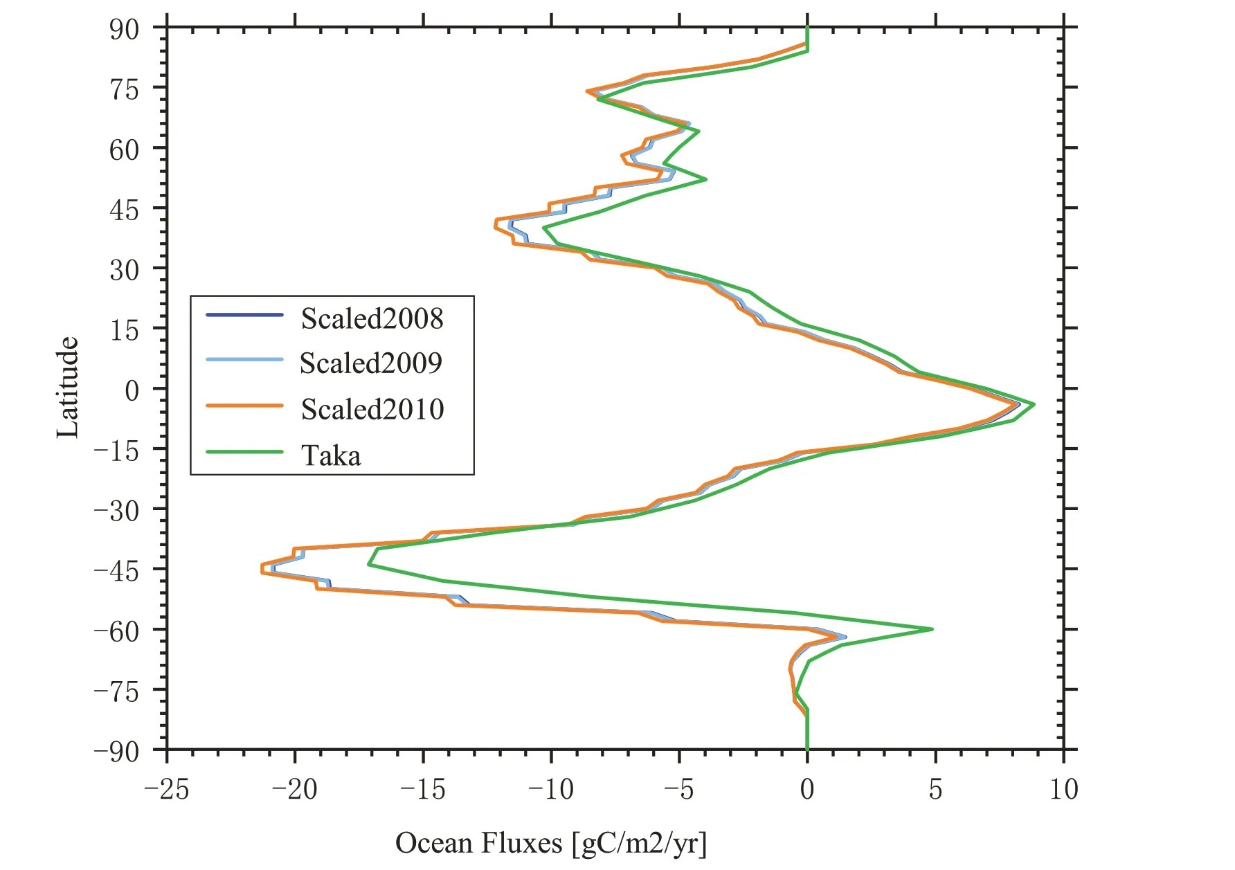
Figure 2. Comparison of the ocean fluxes at different latitudes for 2008-2010.
3.2 The impacts of the ocean carbon flux on the CO2 simulation
Figure 3 presents the differences in the simulated seasonal mean surface-layer CO2concentrations using the two kinds of ocean flux. The simulated CO2concentrations driven by the Scaled Ocean were lower in each season, because the Scaled Ocean carbon flux showed an increasing tendency to absorb CO2each year. From the perspective of the global spatial distribution, there were significant meridional differences,especially in the Southern Hemisphere. The largest difference between the two simulations occurred in autumn(Figure 3(d)),in which the simulation value of the ocean flux with interannual changes was at 0.8 ppm or more in the middle and high latitudes of the Southern Hemisphere. This is related to the large difference between the two kinds of ocean carbon flux in autumn (Figure 1(g,h)). The difference in the two simulated concentrations was relatively weak in winter (Figure 3(a)), and the zonal extreme was around 60°S. In the Northern Hemisphere, the simulated concentration in the ocean was significantly greater than that over land.This shows that the ocean carbon flux has a greater impact on the atmospheric CO2of surface water and is then transmitted through the air to affect the land.
Comparing the simulated monthly surface-layer CO2concentrations with observations,the difference between the simulation results was apparent(Figure 4).The longer the simulation time was,the more obvious the difference between the two simulated results(Figure 4(a,g)),and the closer the simulated values of the ocean carbon flux with the interannual variation were to the observed values.Table 2 provides the RMSE analyses, comparing nine observation sites.The RMSE for the simulation driven by the Scaled Ocean flux was smaller at all stations,indicating that these results were more accurate.The RMSE for CGO station was only 0.583,while the RMSE for the simulation of the climatological ocean carbon flux reached 1.332.Nevertheless,the results of the two kinds of simulation both had a large RMSE at HUN station, while the simulation of the Scaled Ocean was close to the observations.

Figure 3.Differences in the simulated seasonal mean surface-layer CO2 concentrations using the scaled ocean and Taka ocean fluxes for 2008-2010.
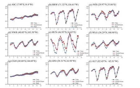
Figure 4.Comparison of the simulated monthly surface-layer CO2 concentrations using the scaled ocean and taka ocean fluxes with observations for nine sites.

Table 2. The RMSE for the simulated CO2 concentrations at nine observation sites (units: ppm month-1).
4. Discussion and conclusion
This study analyzed the seasonal differences in the spatial distribution of the multi-year average ocean carbon flux with interannual changes and the climatological ocean carbon flux,and compared the differences in the simulated global CO2concentration driven by these two kinds of ocean flux from 2008 to 2010. The following conclusions were obtained:
First, over the eastern equatorial Pacific and Atlantic oceans,there are obvious characteristics of CO2release,while the carbon sink located at mid-latitudes and the carbon flux intensity in these regions change with the seasons. The seasonal spatial distribution of the differences in the two kinds of ocean carbon flux mainly depends on the strength of the carbon source; the ocean flux with interannual variability shows weaker release of CO2along the equatorial Atlantic Ocean in summer, 60°S in autumn, and 60°N in the spring, while it takes up more CO2at mid-latitudes.
Second,the CO2concentrations simulated by different ocean carbon fluxes show obvious seasonal differences,which are mainly changes with latitude. The simulation results of the climatological ocean carbon flux are higher,especially in the Southern Hemisphere. Comparing the four seasons, the simulation difference was largest in autumn and smallest in winter.In addition,the simulation differences in ocean regions are relatively higher than those over continents, and this reflects the fact that the main area influencing the ocean carbon flux in the simulation results is the ocean.The comparison of the monthly simulation values and the CO2concentration observed at the nine stations shows that the difference between the two simulation results increases with time.Comparing the RMSE of the simulation values, all of the errors of the simulated CO2concentrations using ocean carbon fluxes with interannual changes were smaller,indicating that the simulation results were more accurate.
Disclosure statement
No potential conflict of interest was reported by the authors.
Funding
The work was partially supported by the National Key Research and Development Program of China [grant number 2016YFA0600203], and the National Natural Science Foundation of China [grant number 41575100].
 Atmospheric and Oceanic Science Letters2019年5期
- Atmospheric and Oceanic Science Letters的其它文章
- Enhanced correlation between ENSO and western North Pacific monsoon during boreal summer around the 1990s
- Contribution of El Niño amplitude change to tropical Pacific precipitation decline in the late 1990s
- Sub seasonal variations of weak stratospheric polar vortex in December and its impact on Eurasian air temperature
- Long-term changes in wintertime persistent heavy rainfall over southern China contributed by the Madden-Julian Oscillation
- Contribution of El Niño amplitude change to tropical Pacific precipitation decline in the late 1990s
- State of China's climate in 2018