Using Kalman filter algorithm for short-term traffic flow prediction in a connected vehicle environment

Azadeh Emami· Majid Sarvi · Saeed Asadi Bagloee

Abstract We develop a Kalman filter for predicting traffic flow at urban arterials based on data obtained from connected vehicles.The proposed algorithm is computationally efficient and offers a real-time prediction since it invokes the connected vehicle data just before the prediction period.Moreover, it can predict the traffic flow for various penetration rates of connected vehicles (the ratio of the number of connected vehicles to the total number of vehicles). At first, the Kalman filter equations are calibrated using data derived from Vissim traffic simulator for different penetration rates, different fluctuating arrival rates of vehicles and various signal settings. Then the filter is evaluated for a variety of traffic scenarios generated in Vissim simulator.We evaluate the performance of the algorithm for different penetration rates under several traffic situations using some statistical measures. Although many of the previous prediction methods depend highly on data from fixed sensors(i.e., loop detectors and video cameras), which are associated with huge installation and maintenance costs,this study provides a low-cost mean for short-term flow prediction only based on the connected vehicle data.

Keywords Connected vehicle · Flow prediction · Kalman filter · Vissim simulator

1 Introduction

Traffic congestion takes a massive toll on cities’ economies. The congestion cost for Sydney and Melbourne is around $6.1 billion and $4.6 billion a year, respectively,and it is projected to increase twofold by 2030 [1]. To tackle the problem of traffic congestion, intelligent transportation systems (ITSs) are considered as an appropriate choice to provide a reliable transport network [2]. To this end,adaptive traffic control is perceived as a useful tool in the ITS toolbox designed to allocate a fair amount of green times to vehicles in signalized intersections. The successfulness of adaptive traffic control strategies depends highly on the accuracy of the input data. Hence, it is essential to enhance the efficiency of traffic prediction algorithms by providing more exact and real-time data. In addition to adaptive traffic signals,traffic prediction is also used in the advanced traveller information system (ATIS), emergency response system planning, variable message signs (VMSs)and real-time route guidance to assist drivers to select the best route among the existing alternatives [3, 4]. The data from various sources such as fixed sensors or floating sensors can be used as input for prediction algorithms.

With the emergence of the connected vehicle (CV)technology,traffic states can be predicted with much higher accuracy in comparison with point detectors such as loop detectors and video cameras since point detector sensors can only provide information about specific spots of a much larger network.Connected vehicles can transmit their information such as position, speed and acceleration/deceleration to other connected vehicles (V2V) and an installed infrastructure near the intersections (V2I) on a real-time basis. Moreover, the data from CVs can also be used to develop smart and intelligent control schemes for a network of signalized intersections. Some CV testbeds are underway around the world to test various applications of connected vehicle technology in the real world [5].

‘‘Connected Vehicle’’ is no longer a distant idea or technology;it is currently becoming a new norm and reality.Recently, some car manufacturers have started to install an on-board unit (OBU) in their new products. The OBU is a small gadget for sending and transmitting signals that can be easily installed inside vehicles.The cost of OBU is no more than a few hundred dollars,and it is projected to decrease in the coming years [6]. The aim is to provide the possibility for vehicles and infrastructure to cooperate to enhance safety,mobility and environmental sustainability.However,there is evidence to support the idea that it takes a long time for new technology such as OBU to become available in all new vehicles and even longer for that technology to be in the majority of vehicles on the road[7].Therefore,there is a need to develop traffic signal control strategies based on data from various penetration rates of connected vehicles,for which one prerequisite is to create accurate and versatile traffic prediction methods.

Moreover, traffic state estimation in a dense city with interlock intersections is a more complicated task compared to freeways and corridors. Nevertheless, a clear majority of research studies in traffic prediction methods are dedicated to traffic prediction in isolated freeways and arterials.

Based on a comprehensive review of the previous studies, developing short-time prediction methods, which use the CV data, is still an open research area. Therefore,this paper presents a Kalman filter strategy to predict traffic flow on a real-time basis using data from CVs. The proposed method does not depend on the data from fixed sensors such as loop detectors. Moreover, it can work for various penetration rates of connected vehicles.The model is also applied to estimate the traffic flow for urban arterials where the signalized intersections can considerably affect the flow of vehicles approaching each intersection.

The paper is organized as follows. The next section is dedicated to the review of the existing traffic state prediction algorithms.In Sect. 3,the methodology of the flow prediction algorithm based on Kalman filter method is explained in detail.Section 4 presents the numerical results of the Kalman method for different penetration rates of connected vehicles as well as various traffic conditions.The conclusion and future research direction are presented in the last section.

2 Literature review

Regarding various prediction models used in the literature,the traffic prediction methods can be classified as parametric, nonparametric and a combination of both.

Parametric models use the training data to adjust some finite and fixed set of parameters of the model and then use the model to estimate the traffic states for a set of different test data.For instance,a family of time series models[8,9]such as linear regression model [10], autoregressive integrated moving average (ARIMA) [11] and Box-Jenkins time series model [12], Kalman filtering and particle filter models [13-15] are types of parametric models.

On the other hand, nonparametric models assume that the distribution of data cannot be easily defined by a set of fixed and finite parameters in the model. Some nonparametric models include neural networks [16, 17] and nonparametric regression models [18, 19]. Some prediction models are developed based on a combination of both parametric and nonparametric models,such as fuzzy-neural network [20, 21], neural network and ARIMA model [22],autoregressive moving average with exogenous input(ARMAX) [23] and machine learning and neural network[24].

Although nonparametric methods show better accuracy in comparison with simple parametric methods such as time series, they require a high computational effort.Moreover,their accuracy is highly dependent on the quality and quantity of the training data [25].

The Kalman filter which uses a state-space model is a popular tool for short-term traffic prediction thanks to its multivariate characteristic, in a sense; there exist several checkpoints to round up noisy data [26]. It can be used in both stationary and non-stationary traffic conditions (in other words, stable and highly volatile traffic circulation).In each step of the prediction,the state variables(which we aim to predict their quantity in our present work) will continuously be updated using the new and real-time traffic condition data collected from different sources [27,28].In this paper,a Kalman filter is developed to predict the traffic flow of each movement approaching an intersection using data gathered from connected vehicles in the previous step of the prediction time.

Prediction data can be obtained from stationary sensors such as loop detectors, radar and video cameras [3, 29] or non-stationary sensors such as GPS devices,mobile phones and probe vehicles [30].

Over the past decade, most research in traffic state prediction has mostly focused on data gathered from single point detectors such as inductive loop detectors [31];however,the prediction of traffic states based on data from connected vehicles is still a new area of research and needs to be more investigated.The poor performance of previous traffic forecasting algorithms based on loop detectors is mostly due to the lack of widespread deployment of these sensors in the area of measurement [32]. Moreover, point detectors can only provide information about specific spots and therefore are not able to reflect the real situation of the traffic in the whole network [33]. These sensors are also associated with huge installation and maintenance costs[34].With the emergence of connected vehicle technology,it is possible to collect information from connected vehicles in various parts of the network. This precise information can be obtained several times in a second. More accurate data can give rise to better accuracy of the prediction models[35].One major drawback of this approach is the imperfect penetration rate of connected vehicles;recent studies have shown that even if US car manufacturers are mandated to install OBU on light vehicles, it takes approximately 25-30 years to have 95% of vehicles equipped with communication devices [36]. This implies the need to develop prediction methods based on a limited number of connected vehicles [37, 38].

We can summarize the above discussion as follows:

· To optimize the parameters of adaptive traffic signal controllers, it is of critical importance to predict the traffic flow for short intervals (i.e., real-time traffic prediction). Relatively long intervals cannot be used to accurately adjust the traffic controller parameters in accordance with the short-term variation of the traffic condition.However,a vast majority of the literature on traffic forecasting is dedicated to long-term traffic prediction. Hence, it is necessary to develop new algorithms able to accurately predict the traffic state for a short-time horizon toward the future.

· Over the past decade, most research in traffic forecasting has emphasized the prediction of traffic flow in freeways and corridors;however,the urban traffic flow prediction is a more complex problem in the heart of cities with interlock signalized intersections [32].

· A considerable amount of traffic forecasting literature has developed their methods based on data gathered from stationary sensors such as inductive loop detectors. With the emergence of CV technology, it is possible to have access to more accurate data from connected vehicles, so there is still an open area for research in the use of connected vehicle data to predict traffic states.

· Since it is predicted that reaching a 100% penetration rate of connected vehicles is not in the scope of near future, it is of vital importance to develop prediction methods that can predict the traffic situation based on data from a limited number of CVs [39].

Based on the aforementioned knowledge gaps, this paper aims to develop a short-term traffic prediction algorithm to predict the flow of vehicles in urban networks based on only data from a limited number of connected vehicles.

3 Methodology

Consider multi-approach traffic stream flows toward an intersection as shown in Fig. 1.Traffic flow counted at the reference line is the result of merging three traffic streams denoted by F1, F2and F3. The problem is to predict the flow at the reference line using two traffic flow data sources: (1) historical data and (2) a limited number of connected vehicles both pertaining to traffic streams F1,F2and F3.

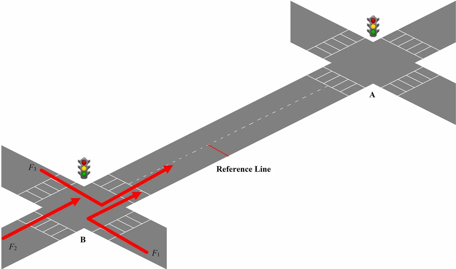
Fig. 1 The layout of the two consecutive intersections

To achieve this, we use a Kalman filter model. In other words, based on the real-time flow information of connected vehicles in each step of the prediction, the flow in the next time step is predicted. In this section, we first introduce the basic concepts of the Kalman filter algorithm followed by a calibration and evaluation process.

3.1 Kalman filter algorithm

The Kalman filter is a state-space model that was first introduced by Kalman [40]. It can be applied to model systems with multi-input and multi-output and can be used for both stationary and non-stationary situations. This feature of the Kalman filter makes it an appropriate choice for modeling the traffic states[3].Kalman filter updates the prediction of state variables based on the observation in the previous step.Therefore,it only needs to store the previous estimate information. The Kalman filter has two distinct features: (1) It does not require any additional space to store the entire previously observed data. (2) It is computationally efficient since it does not need to utilize all the previous estimated/measured data in each step of the prediction process[41].In this study,the Kalman filter is used to predict the flow of vehicles (i.e. state variables) on the basis of the real-time information received from connected vehicles (observation) in the last step of the prediction process.The prediction of the state variable is realized in a recursive procedure in which observations and previous states are used to calculate the flow state for the next step of the prediction process.

Let xkdenote the state variables,which are used to show the flow of vehicles approaching an intersection during the time step k (see the reference line in Fig. 1). The Kalman algorithm is used to predict the xk+1, traffic flow for the next time step. Note that φkrepresents the state transition matrix which maps the previous state xkinto the next state xk+1. We consider a noise vector denoted by wk, with a normal distribution with zero mean and variance Qk. The state prediction model can then be written as follows:

Let zkindicate the observations at time step k,which shows the flow of connected vehicles approaching the reference line, H be a matrix denoting the relationship between the measured variables and state variables, and vkshow the measurement error which is a Gaussian noise with zero mean and variance Rk. Moreover, wkand vkdo not have any correlation and are statistically independent, that means for all i and j, we havedenotes the expected value. Hence, the flow observation may be written as In each step of the prediction algorithm,detailed below,the state variables will be updated using a recursive process:

Step I: Initialization:

Step II: Extrapolation:

Step III: Calculation of Kalman gain:

Step IV: State and error covariance update:

Step V:let k = k + 1 and go back to step II and continue the process until the end of the present time period.

In the next section,the calibration process using the Vissim traffic simulator is presented.

3.2 Kalman filter calibration

In order to construct the state space and measurement equations in (1) and (2), the state transition matrix φk, the measurement mapping matrix H,the noise matrixes wkand vk, which are considered to be scalar in this study, are estimated from ground-truth data.

Note that,xk,the traffic flow approaching an intersection(crossing the reference line) depends on different external factors such as the traffic signal control of the upstream intersections as well as their geometries and layouts.Therefore, the Kalman filter equations need to exclusively adjust for each layout. Although real traffic data is important to evaluate the prediction algorithms,because of the unavailability of CV data at this stage of the study, we use the Vissim data as the ground-truth data. However,since the authors of this article are recently involved in a connected vehicle testbed project in Melbourne, called Australian integrated multimodal ecosystem (AIMES)(https://eng.unimelb.edu.au/industry/aimes), testing the algorithm with the real data from a CV environment is one of the plans for this study. To this end, the data obtained from the Vissim traffic simulator are used as historical data to derive and calibrate the equations. To achieve this, two consecutive intersections are simulated in the Vissim traffic simulator. The flow information of all vehicles including connected vehicles pertaining to different signal settings and arrival patterns and various penetration rates of connected vehicles for 2 h of the simulation is collected. We deploy the MATLAB as a COM interface to control the Vissim simulator. Moreover, the training and test data used, respectively, for calibration and evaluation of the Kalman algorithm are collected through MATLAB. We also realize the Kalman filter algorithm in a MATLAB m.file. The aim is to predict traffic flow for short time intervals toward the future to be used later in traffic signal settings. Here, a time interval of 50 s is considered.

The state transition matrix φkand noise matrix wkare calculated based on a linear regression model on the state variable vector xkand previous state vector xk-1. In order to determine the wk, the variance of the error between the previous state vector xk-1and state vector xkneed to be calculated.

In the measurement Eq. (2), the state variable in each time step is calculated based on the measured variable zk.In this study, zkindicates the flow of connected vehicles travelling from three approaches of the preceding intersection in each step of the prediction period. H maps the number of connected vehicles in the traffic flow to the total flow of vehicles. Note that H is calculated using a linear regression model based on the total number of vehicles in the flow as an independent variable. This coefficient is interpreted as the penetration rate of connected vehicles.Noise variance vkis calculated based on the variance of the error between the measured variable zkand state variable xk. The calibration process is evaluated using three widely used metrics [42, 43], as discussed in the next section.

To predict the flow at the reference line (Fig. 1), the merging traffic flows must be recorded in 50-s time intervals. Hence, the number of connected vehicles passing the reference line every 50-s time interval is recorded and used as input for the Kalman filter algorithm.At first,the flow is predicted for different penetration rates of connected vehicles as well as various traffic signal settings of intersection B, which profoundly affect the flow rate of the reference line. We consider some predetermined and fixed traffic signal plan for upstream intersection B (Fig. 1).Each of these signal plans can be implemented to control intersection B based on its traffic condition. Considering a variety of traffic conditions by changing the signal plan of upstream intersection B will result in dissimilar flow pattern approaching intersection A. Therefore, the Kalman equations can be trained considering variation in the flow patterns.This can result in better accuracy of the algorithm to estimate the flow in different traffic situations.To do so,it is needed to calculate the arrival times of the connected vehicles. As such, the connected vehicles’ information such as their positions, speeds, and acceleration/decelerations will be available in different time steps during the prediction horizon. This information is available in the basic safety message that will be sent to the roadside unit devices via dedicated short-range communication (DSRC)platform ten times per second by vehicles equipped with on-board unit(OBU)devices.Therefore,we need to collect three types of data from connected vehicles including position, speed and acceleration/deceleration to be able to calculate the arrival time of each connected vehicle to the reference line. From this information and based on the following formula,the arrival time of connected vehicles at the reference line can easily be calculated. Therefore, we can then count the number of connected vehicles that cross the reference line in each time step of the prediction based on their arrival time:

where xpis the position of the reference line, a is the acceleration/deceleration, v0is the current speed, x0is the current position of the target connected vehicle,and t is the remaining time for the vehicle reaching to the reference line. In order to estimate the time of arrival with a better accuracy, t can be updated in each time that a new information is available from connected vehicles.Notice that to estimate the flow for each different reference line, the Kalman filter parameters need to be calibrated based on the flow characteristics and layout of the upstream intersection. To use the flow prediction results in adaptive traffic signal controllers, we could use a parallel computation for all reference lines. The pseudo-algorithm represented in Fig. 2 describes the process of calibration and evaluation of the Kalman algorithm.At first,the Vissim simulation is run for a sufficient number of times to populate the network(warm-up period); then for each penetration rate of CVs,the simulation is run for a random pattern of vehicle inputs and signal plans of the upstream intersection.Then the flow and CV information are collected via MATLAB.This data is deployed to calibrate the state and measurement equations of the Kalman filter. After that, we generate random traffic situations, run the Vissim for one step and measure the CV data. In the next step, The CV data is deployed in the Kalman filter algorithm to predict the flow for the next time step. The prediction algorithm is run for a sufficient number of times (a desired value). To be able to evaluate the performance of the proposed algorithm, we need to determine the total number of samples that can be used to validate the Kalman algorithm.This predetermined number of time-steps in this paper is called the desired value. This desired value should be sufficiently big to provide an unbiased evaluation of the performance of the Kalman algorithm. The estimation results of the algorithm for all time steps are then compared with the real flow derived from Vissim simulation.

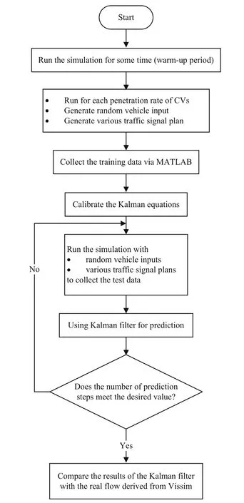
Fig. 2 The pseudo-algorithm for traffic flow prediction based on Kalman filter

The information on the case study layout is summarized in Table 1. We consider Poisson arrival rates for vehicle inputs in each approach of the intersection. The rates of vehicle inputs are randomly changed;however,on average ten vehicles cross the reference line in each 50-s time intervals.

Table 1 The summary of the case study information

4 Numerical results

Here in this section, the performance of the Kalman filter method is tested for various ranges of CVs. Moreover, the prediction results are compared for normal traffic condition as well as for the condition with sudden changes in the flow pattern.Three performance criteria are used to evaluate the performance of the proposed Kalman filter method, rootmean-square error (RMSE), mean absolute error (MAE)and mean absolute percentage error (MAPE):

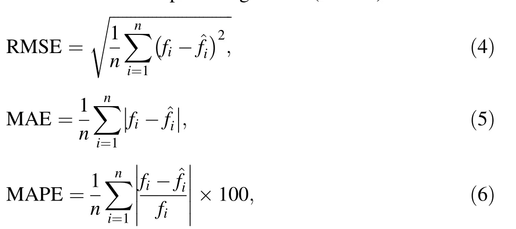
where fiandeasured at each time step of the prediction are the real and predicted traffic flow, respectively. Note that i is the index of the time interval and n indicates the total number of observation and prediction of flow.

In order to illustrate the performance of the proposed flow prediction method, the method is evaluated under various penetration rates of connected vehicles and different congestion levels.

Figure 3 indicates the traffic flow prediction for different penetration rates of connected vehicles while considering various traffic signal settings of the intersection B.As shown in Fig. 3, as the penetration rate increases, the Kalman filter provides better and accurate prediction results. The vertical axis represents the total number of vehicles that cross the reference line during each time step(say 50 s). The horizontal axis shows the estimation time steps. Each estimation time step is equal to 50 s.

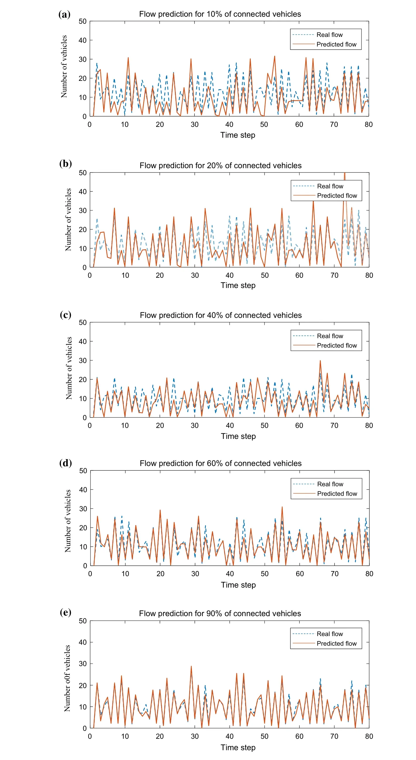
Fig. 3 Flow prediction for different penetration rates of connected vehicles

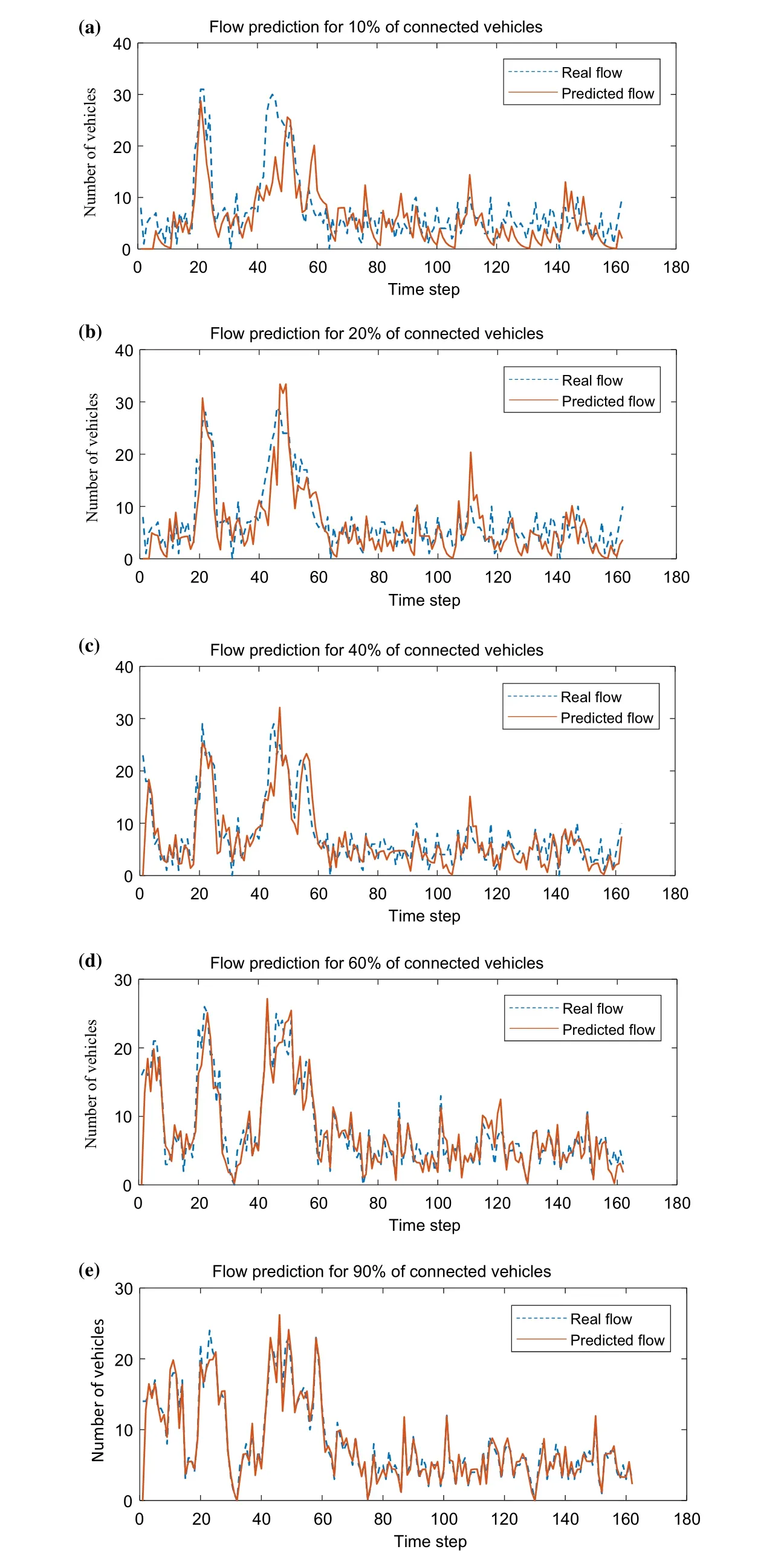
Fig. 4 Flow prediction for different penetration rates of connected vehicles and abrupt changes in flow pattern

In this study, we also evaluate the performance of the proposed Kalman filter technique to track the abrupt changes in the traffic condition. Here we assume that the data related to the sudden changes in traffic flow are not considered in the adjustment of the parameters of Kalman filter equations. The aim is to evaluate the performance of the Kalman filter when there is a considerable change in the flow of vehicles.In order to do so,at first,the Vissim traffic simulator will be run for an undersaturated traffic condition.Then two times it was suddenly converted to saturated traffic condition (the average flow of vehicles in this stage is two times more than the undersaturated condition) by changing the number of input vehicles at intersection B in Fig. 1.Each time after rising the flow,the traffic condition again turns to the undersaturated traffic condition. Therefore, we can make a fluctuation in the traffic and evaluate the ability of the Kalman filter to track the changes. The connected vehicle data from Vissim is used to predict the flow of vehicles based on the Kalman filter method. One may argue for expanding the reach of the proposed algorithm to include autonomous vehicles’ data.To this end,it is important to note that a driver-less car basically is a car without a driver and hence is not necessarily a connected vehicle. An autonomous vehicle can be considered a connected vehicle only if it is equipped with on-board unit(OBU)and it can communicate with roadside units(RSUs)and other vehicles. Take for example the famous Google car which is an ad hoc autonomous vehicle and it is noted connected to anywhere (Google’s Autonomous Vehicle,2017). In the situation where autonomous vehicles are equipped with communication devices, we can easily consider them as connected vehicles in our methodology.

Results for the measured flow as well as predicted flow are shown in Fig. 4. Since an increase in the flow of all vehicles in the network results in a rise in the flow of connected vehicles, the measurement equation can track the changes in the flow of vehicles. Even for the situation that the covariance noise of state and measurement equations are gathered exclusive of considering the huge changes in traffic flow, results of the flow prediction algorithm are still satisfactory. Therefore, the proposed algorithm has the capability to trace the flow even with the abrupt changes in the traffic flow pattern.

Table 2 presents a summary of statistical metrics pertaining to various penetration rates of connected vehicles for two distinct scenarios: (1) normal traffic condition and(2) when abrupt changes happen in the traffic flow. As expected, R-squared is improved as the number of connected vehicles increases. Similarly, there exists a clear trend of improvement in all error indices as the penetration rate of connected vehicles rises. In other words, the Kalman filter works much better in situations with more connected vehicles. Figure 5 represents the R-squared for normal traffic condition (undersaturated) and abrupt changes (saturated). As can be seen, the paces of changes in both saturated and undersaturated cases are confirmative.Moreover, the strength and merit of the Kalman filter are shown when it can effectively detect and handle abrupt changes because the Kalman filter adaptively predicts the flow based on the real-time information from the present traffic situation.

It is important to note that the Kalman filter is a frugal model,in the sense that,it does not need a high number of connected vehicles to perform well. As can be seen in Fig. 5, the penetration rate of at least 20% is a commensurate and healthy choice for the Kalman filter. This is a compelling result that proves the effectiveness of the proposed Kalman model to predict the flow for a low market penetration rate. For the penetration rate of 60% or more,there exists only a marginal improvement in the performance criteria. Therefore, for the reasonable and accurateperformance of the proposed prediction algorithm, there is no need to have a near perfect market penetration rate(around 100%).

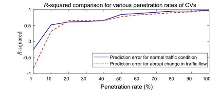
Fig. 5 RMSE and R-squared comparison for normal traffic condition and abrupt change in flow across various penetration rates of CVs

5 Conclusion

This paper presents a Kalman filter technique to predict traffic flows approaching an intersection based on the data of connected vehicles. At first, parameters of the Kalman equations are adjusted through the use of Vissim microscopic traffic simulator.Then,we evaluate the performance of the model for different penetration rates of connected vehicles under various traffic conditions. The results obtained from this study show the Kalman filter performs well when the penetration rate is more than 20%.

We also test the accuracy of the model to track abrupt changes in the traffic condition and show the effectiveness of the model based on several error indexes. It is apparent from the results that the proposed method has an acceptable accuracy to predict the traffic flow even in the presence of abrupt changes in traffic condition.Moreover,there is a positive correlation between the model’s accuracy and the penetration rates, in the sense that, as the penetration rate increases, the model predicts traffic flow with more resolution.

Future work should focus on the improvement of the algorithm tailored to situations in which the penetration rate is significantly low.For instance,we could also use the data from inductive loop detectors and Bluetooth data to predict the flow with more accuracy under low penetration rates. Moreover, to predict the flow with higher accuracy,we can consider the traffic signal states of upstream intersections as input variables in the state equation of the Kalman filter.Testing the accuracy of the algorithm against ground-truth data from the real world connected vehicle testbed is one of our focuses for future study. Moreover,the estimation algorithm can also be integrated into an adaptive traffic signal plan [44] to control the traffic based on the real situation of the traffic in the network.

AcknowledgementsThis work has been sponsored by the Australian Integrated Multimodal EcoSystem (AIMES), https://industry.eng.unimelb.edu.au/aimes. The authors would like to thank many industry and government partners, in particular, Cisco, CUBIC, Cohda Wireless, VicRoads, Department of Transport, Traffic Accident Commissions, and PTV Group. The authors would like to thank Prof Zhai, the editor in chief and two anonymous reviewers for their constructive and insightful comments.

Open AccessThis article is distributed under the terms of the Creative Commons Attribution 4.0 International License (http://creativecommons.org/licenses/by/4.0/), which permits unrestricted use,distribution,and reproduction in any medium,provided you give appropriate credit to the original author(s) and the source, provide a link to the Creative Commons license, and indicate if changes were made.