Embedded model control:Reconciling modern control theory and error-based control design

Enrico CANUTO,Carlo NOVARA,Luigi COLANGELO

Politecnico di Torino,Italy

Received 27 June 2018;revised 23 July 2018;accepted 23 July 2018

Abstract

The paper addresses the problem of reconciling the modern control paradigm developed by R.Kalman in the sixties of the past century,and the centenary error-based design of the proportional,integrative and derivative(PID)controllers.This is done with the help of the error loop whose stability is proved to be necessary and sufficient for the close-loop plant stability.The error loop is built by cascading the uncertain plant-to-model discrepancies(causal,parametric,initial state,neglected dynamics),which are driven by the design model output and by arbitrary bounded signals,with the control unit transfer functions.The embedded model control takes advantage of the error loop and its equations to design appropriate algorithms of the modern control theory(state predictor,control law,reference generator),which guarantee the error loop stability and performance.A simulated multivariate case study shows modeling and control design steps and the coherence of the predicted and simulated performance.

Keywords:Modern control theory,error-based design,embedded model control,error loop,disturbance rejection

1 Introduction

In the 80’s of the past century,J.Han of the Chinese Academy of Sciences,Beijing,China,in a suite of Chinese-written papers(see[1]for a more recent English summary)pointed out the difficulties of themodern control paradigmproposed by R.Kalman in his seminal paper“On the general theory of control systems”[2]in front of the real plant uncertainty.Z.Gao observed in[3]that the robust control design is apara-doxthat looks unsolvable within the modern control paradigm.The stunning fact is that,after sixty years of modern control theory and myriads of publications,the proportional,integrative and derivative(PID)controller,formulated around 1920 and applied to ship steering by[4,5],is still the work-horse of automatic control in all the fields of application.The argument of J.Han and Z.Gao[1,3,6]is that PID design and tuning(theerror-based design paradigm)is substantially model independent and only guaranteed by the experimental per-formance of the measured tracking error between reference and plant measurements.It seems evident that a fracture exists between a well-established and mature mathematical theory and a centenary successful engineering practice.

Is a reconciliation workable and by which means?The goal of this paper is to prove that reconciliation is feasible and that robust control theories and design methodologies exist and have been in-field applied.The main design objective is to guarantee stability and performance of a real control system in the presence of a given class of uncertain discrepancies between real plant and mathematical model.

The key result of the paper in Section 2.3.3 is that,given a suitable mathematical model of the plant and the required performance,Kalman theory allows a class of parameterized controllers to be designed and tuned in order to guarantee stability and performance in presence of a well-defined class of uncertain discrepancies.The tool for controller tuning and performance verification is theerror loop[7],in which plant and model discrepancies are appropriately filtered by the controller itself for guaranteeing stability and requirements.A theorem proves that the error loop stability is a necessary and sufficient condition for the stability of the closed-loop plant.

The paper is organized into three steps.

Section2 starts by briefly recalling Kalman theory and objectives[2]and the unstructured uncertainty defined by the robust stability theory of J.C.Doyle and G.Stein[8].Both theories together with the smallgain theorem of G.Zames[9]are the foundations of the theory of F.Donati and M.Vallauri[10].The theory exploits the machinery of the input-output norm of dynamic operators to define concept and method of“almost-linear plants”.In essence,the output error norm between almost-linear plant and model can be made smaller than the model output norm:in other terms,the fractional error can be brought to be less than 100%.Though insufficient to invoke the small-gain theorem for the whole loop including plant and controller,it facilitates the model-based design of a feedback controller that guarantees a loop gain less than unit and therefore closed-loop stability.The stabilizable loop,referred to as the error loop in[7],is proved to be the cascade of the unstructured uncertainty and of two model-based closed loop transfer functions.

Section3 traces the path from Section2 to the embedded model control(EMC)[7,11].First it goes beyond the unstructured uncertainty by separating four uncertainty classes:initial state,parametric and causal uncertainty and neglected dynamics,and proves that whereas parametric and causal uncertainty must be canceled on the plant,neglected dynamics contribution must be blocked from entering the controller itself.The controller architecture is similar to that of F.Donati and M.Vallauri[10]as well as to the internal model control[12]and the active disturbance rejection control[3].As a second point,design and embedded model are distinguished.The design model,which surrogates the plant,includes the whole uncertainty class.The uncertainty simplifies to the causal uncertainty in the embedded model,which is the core of the controller and is the basis for the controller design.Design model and controller allow to build design equations which relate tracking and other errors to the uncertainty class elements(the error loop equations)and guide the robust controller tuning(pole placement)through analytic inequalities relating requirements,controller parameters(closed-loop poles)and uncertainty bounds.

Models,equations and pole placement of Section3 are employed in Section4 to solve a well-known multivariate and nonlinear control problem[13],which does not admit the normal form of the feedback linearization[14]and is non-minimum phase in the linear approximation.Analytic design versus uncertainty is checked by simulated trials.

2 The robust design problem

2.1 R.Kalman’s theory

In his seminal paper on the“General theory of control systems”[2],R.Kalman’s ultimate objective was to answer two questions:

1)What kind and how much information are needed to achieve a desired type of control?

2)What intrinsic properties characterize a given unalterable plant as far as control is concerned?

The aim is that of“initiating study of the pure theory of control,imitating the spirit of Shannon’s investigations in the theory of information”,but “avoiding the well known difficulty of Shannon’s theory:methods of proof which are impractical for actually constructing practical solutions”.To this end,“only constructive methods are employed”but restricted to “dynamic systems with a finite dimensional state space and linear transition functions,excited by an uncorrelated stationary Gaussian random process”.R.Kalman did not explicitly answered the above questions but proved that“the general problem ofoptimal regulationis solvable if and only if the plant iscompletely controllable”,and that“the optimal state predictionwhich solves the Wiener filtering problem”requires thecomplete observabilityof a linear dynamic system excited by a Gaussian random process.The concepts ofplant(“physical object”)andmathematical model(“dynamic system”)are distinguished;but the paper concentrates on the model properties with the explicit assumption(page 482,[2])that model input and output are at the same time plant input and output.Theinherent uncertaintyof the input and out put random processes is just seen as a model(and plant)property.

Sufficient conditions for linear time-invariant(LTI)model stabilizability.In summary,although not explicitly stated and by confounding plant with model,controllability and observability(brieflyminimality)are proved to besufficientconditions for designing asymptotically stable(AS)LTI regulators and predictors,andnecessary and sufficientfor their optimality,independently of the uncorrelated stationary Gaussian random processes(with bounded covariance in the discrete-time(DT)case and bounded spectral density(SD)in the continuous-time(CT)case)which are applied to the model.Minimality is only sufficient for the stabilizability since also non minimal LTI models may be feedback stabilized.

2.2 Doyle-Stein’s robust stability

A first step toward a theory ofuncertain dynamic systemsand their stabilizability was done in 1981 by J.C.Doyle and G.Stein[8].The input-output LTI design model expressed by the minimal transfer matrixM(s=j2πf),f≥ 0(without pole-zero cancellation),is complemented by an unknown but bounded perturbation ΔP(jf),whose bound is defined by the set membership statement:

wheref≥ 0 and σmaxis the largest singular value of ΔP(jf).The uncertainty defined in(1)which does not postulate any specific expression of ΔP(jf)is referred to asunstructured uncertainty.Since matrix algebra admits multiplication(though not commutative),the authors of[8]recognized that uncertainty can be expressed in a multiplicative way as

where,ifMis invertible,the form

takes the meaning of afractional/relative error.Comparison of the set membership uncertainty in(1)with the uncertainty of a stationary Gaussian random process postulated by the R.Kalman theory in[2],though of interest,is left to the reader.

Sufficient conditions for robust LTI stabilizability.Given a feedbackF(jf)that stabilizes the closed-loop complementary sensitivity(CS)V(jf)defined byV=(I+FM)−1FM,and the additional assumption of equal number of unstable poles inFPandFM,the “robust”closed-loop sufficient stability condition amounts to the small-gain inequality:

2.3 Donati-Vallauri’s robust control theory and the Han’s paradox

2.3.1 The input-output unstructured uncertainty

A further step was made in 1984 by F.Donati and M.Vallauri[10]by defining the unstructured uncertainty in terms of the input-output norm of dynamic operators(not necessarily linear)and by employing the same machinery of thesmall-gain theorem[11]of G.Zames[9].In this framework,given,for instance,the finite norm of a time-truncated vector signal:

where|v(τ)|is the vector Euclidean norm,a dynamic systemy=P(u)is said to befinite-gain stableif there exists a pair?η,δ?of finite reals such that

where,in the sequel,‖·‖= ‖·‖2,Hunless otherwise said.Time truncation corresponds to the frequency resolution Δf≥H−1.i)Given a real plant(distinguished from mathematical models)defined by an unknown input output operatory=P(u)and an admissible input set U;ii)given a minimal linear dynamic modelym=Mu(respecting causality)and the model errorm=y−ym,plant and model admit anunstructured uncertainty,if and only if a finite pair?ηP,δP?exists such that

In[9]and[10],the input-output operators map time signals defined in a Banach space[15].Here,we restrict to a Hilbert space[15]defined by the scalar product＜v,w＞of the complex vectorial functionsvandwfor any finite 0≤H＜∞:

wherev∗is the transpose conjugate ofv.In the LTI case and in the Hilbert space,the input-output norm of a dynamic operatorMis defined in the frequency domain by

The operator norm ‖·‖∞is known as theH∞norm and σmaxdenotes the largest singular value.In the following,the supremum sup will be changed into maximum max by slightly shifting the imaginary axis poles into the left half-plane.

As in(3),we prefer converting(8)into a fractional uncertainty,by replacing ‖u‖with ‖ym‖.This requires the replacement ofuwithyminP(·)and the approximate inversion ofMby means of a suitable feedbackFuas in Fig.1.

As a result,the input set U becomes restricted to the subset

whereVu=(I+FuM)−1FuMis AS and,being a complementary sensitivity,plays the role of a low-pass(LP)filter capable of attenuating the high-frequency(HF)components ofu.This is the dual effect of the time truncation in(5),since the frequency bandwidth(BW)fuofVuconstrains the time resolution Δtofuto satisfy Δt≥1/(2fu).IfMis a DT model with time unitT,the inverse approximation is accurate as soon as Δt＜T.It is now possible to define thefractional error operator∂P(ym):

and to redefine theunstructured uncertaintyby means of the following input-output norm inequality:

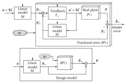
Fig.1 Block diagram of the fractional error operator.

In the light of(4),an uncertainty defined by

and implying σmax(V(jf))≤ 1/η ＜ 1,is such to contrast the sensitivity performance requirement σmax(S(jf)) ≤1/η ＜ 1,f≤fs,whereS=I−V,as soon asfs＞f∂P,leading to an unfeasible design.

Two questions arise.Which is the source of the in-coherence among model,uncertainty and required performance?Focusing on the model and its uncertainty,is there a criterion for testing model adequacy?

F.Donati and M.Vallauri in[10]approached the problem by extending Kalman theory to robust design,i.e.,by separating control strategies into state observer,feedback control law and reference generator.Under unstructured uncertainty,observer and control law design cease to be independent,but their dependence can be made sufficiently weak.Let the control performance be defined by the norm ‖Wr(r−y)‖of the weighted tracking errorWr(r−y),wherer∈R is the reference signal belonging to a set R of the Hilbert space defined by(8)andWris a LP filter.

2.3.2 First design step:the almost-linear plant

The first design step is to look for analmost-linear plant=(u)with the following properties:

1)The unstructured uncertainty inequality,to be compared with(12),holds

where=−ymis the model error of the almostlinear plant and η＜1 in agreement with the small-gain theorem[11].In(14)we took the liberty,justified byT＞ Δt≥1/(2fu),of assumingym=andu=u∗.

2)Thenorm‖Wr(r−)‖of the weighted tracking errorWr(r−)of the almost-linear plant,can be made arbitrarily small by the second design step in Section2.3.3.

Real and almost linear plants are shown in Fig.2.

The first property can be achieved by filtering theopen-loop model errorin(11),now rewritten asm=y−ym,through the CSVm=(I+MFm)−1MFmof an AS state observer.The observer is built aroundMby means of a feedback operatorFm,which is driven by themeasured model error em=y−(see the left-hand side(LHS)of Fig.2).Controllability and observability ofMare sufficient conditions for this design.Let us writein terms of the observer sensitivitySm=(I+MFm)−1and of the CSVm=I−Sm,i.e.,

The right-hand side(RHS)identity of(15)allows the inequality(14)to be rewritten with the same variables of(12)as follows:

Further,sinceVmis a LP filter,(16)proves that an ASstate observer can attenuate the norm of the open-loop model error=y−ymdown to the norm of the almostlinear plant model error(alsoclosed-loop model errorandprediction errorin Section 3).

Fig.2 Equivalence between a plant with a state observer and the almost-linear plant.

The LHS block-diagram in Fig.2 shows plant and state observer,both driven byu.Equation(15)allows us to draw the RHS diagram which shows how plant and model contribute to.For later use(see Section 3.1),the outputdof the dynamic feedbackFmplays the role of aninput disturbanceadding to the command.This interpretation has been exploited by the EMC(see[7]and[11])and by the Active Disturbance Rejection Control(ADRC)[3]in the design ofFm,with the aim of canceling theunknown componentsofdfrom the plant.We also define the output disturbance

which is common in the classical control design.Thus,can be rewritten as

Since,given a controllable and observableM,a family of AS state observers with different filtering capabilities can be built,given a plantP,the design of an adequate modelMis anecessary conditionfor the construction of an almost-linear plant satisfying(16).In other terms,givenPandM,noVmmay exist that guarantees(16).The statement justifies Kalman’s theory(themodern control paradigmin[3])and contradicts the ubiquitous univariate PID feedback,whose design is substantially model independent and only guaranteed by the experimental performance of the measured tracking errore(t),as pointed out by J.Han and Z.Gao in[1,3,6](what they call theerror-based design paradigm).The work of J.Han on the difficulties of the modern control paradigm in the real plant control design dates back to the 80’s,but unfortunately his publications were restricted to Chinese language.He observed in[3]that the robust control design is aparadoxthat looks unsolvable within the modern control paradigm.

First of all,as pointed out by the same authors in[1]and[3],the ideal PID law

cannot be implemented as it is,but the errore,its derivativeand the reference signal must be arranged and adequately filtered to better match the simple feedback(19)with plan tuncertainty and irregularities.Second,inequality(16)is a condition on thefractional error operator∂P(ym)defined in(11)and not on the modelM.The second design step of the Donati-Vallauri’s approach will prove that robust control design is concerned with the stability and performance of the so-callederror loop,which was suggested by E.Canuto(2007)in[7]and again in[16]within the framework of the embedded model control.In essence,the argument of this paper is that almost-linear plant and error loop design can reconcile modern control and error-based control paradigms.

A first piece of the error loop is shown in Fig.3,where model and tracking errors propagate along a closed loop.Section2.3.3will show that the stability of the error loop is anecessary and sufficient conditionfor the stability of the real closed-loop system.The loop is driven by the reference signalrand provides thetracking errorin the formr−ym.The cloud driving the fractional error∂Paccounts for arbitrary and unpredictable sources of uncertainty(causal uncertainty)like the random measurement errors in the Kalman’s theory.The block marked by “?”will be the result of the second design step.

Fig.3 A first piece of the error loop.

To conclude,since ∂P(·)is partially unknown and time-varying,inequality(16)cannot be exhaustively proved in the command set U,given that the set∂P of the candidate∂P,though reasonably bounded,is partially unknown.This implies the risk that(16)ceases to be valid,the risk being commonly reduced,but not zeroed,by fixing a gain margin,that is η ≤ ηmax＜ 1.The inverseis known as thegain margin.Anomalous situations can be revealed by the controller itself and require an appropriate control system reconfiguration leading to degraded performance.

2.3.3 Second design step:fundamental theorem and error loop

Although(16)is a well-defined target for the observer design,it isinsufficientfor guaranteeing the closed-loop stability of an arbitrarycontrol lawaround.This is reasonable,since the“small gain theorem”[11]requires that the whole loop operator in Fig.3 possesses a gain less than unit.In terms of the error loop in Fig.3,we are still missing the operator mapping the closed-loop model errorinto the tracking errorr−ym.

The control requirement is formulated by the norm inequality

whereWris a LP filter that was already defined and R is the reference signal set.The feedback design aroundrequires thatappears in(20),which is obtained with the help of(15)and by splitting the weighted tracking error as

whereWr(r−)is the weighted tracking error ofandy−=WrSm(y−ym)is the open-loop model error filtered by the band-pass filterWrSm.The mid-frequency errory−may be referred to as theresidual model errorsince free of low-frequency(LF)components(they are eliminated bySm)and HF components(they are eliminated byWr).In general,the residual model error cannot be brought to zero,since the frequency BW ofWris wider than that ofSm.

We now state thefundamental theorem,which proves the second property of almost-linear plants and justifies their construction.

Fundamental design theoremThe tracking error norm‖Wr(r−)‖can be made arbitrarily small by the control law

which is applied to the almost-linear plant defined by(18)under the sufficient conditions:

The first condition states that the loop gain η‖Vc‖∞must be less than unit(bounded-input-bounded-output stable closed loop);the second condition states that the gain of the band-pass filterWrSccan be made arbitrarily small by enlarging the frequency BW ofSc(efficient closed-loop control);the third condition fixes the reference gain in(22).The first and second condition are each other contrasting,but the contrast is attenuated by η＜1 as required by the almost-linear plant design in(16).More practical is the lower bound‖WrSc‖∞≥ εr,which is imposed by the command set U(typically|u(t)|≤umax)and in general by technology limitations and cost.EMC exploits these and other contrasting inequalities by generating frequency bands where the bandwidths of the state observer and control law sensitivity,and of their CS,are compelled to stay.When these regions become void,they reveal that the control requirement in(20)cannot be met.The third condition cannot be exactly met,but can be approximated by a wide-band closed-loop inverseCr=VrM−1like in(10).Fig.4 shows the overall closed-loop system which consists of the almost-linear plant in Fig.2 and of the control law(22).

Before completing the error loop in Fig.3,we need to prove the fundamental theorem.

Fig.4 The closed-loop system.

Proof of the fundamental theoremThe proof starts by replacing(22)into(18),which provides

By using the third condition in(23),we obtain the pair of identities

and the pair of inequalities

Replacement of the second inequality of(26)into(16)allows the closed-loop model error=−ymto be expressed in terms ofras follows:

Finally,replacement of the third row of(27)into the first row of(26)provides the expected inequality:

which isboundedunder the first condition of(23)andconverges to zerounder the second condition. □

The error loop in Fig.3 is ready to be completed.The last row of(25)provides the missing operator,the CSVc,which completes the error loop as in Fig.3.Three tracking errors are at the output of the error loop:r−y(from the real plant)andr−(from the almost-linear plant)already appeared in the decomposition of(21),whereasr−ym(from the model)appeared in the second row of(25).Error loop stability can be defined as follows.

Error loop stabilityThe errorloop in Fig.5 is bounded-input-bounded-output stable if for any boundedr∈R all the error loop signals are bounded.

A sufficient stability condition is that

since it implies that‖ym‖and all the other loop signals are bounded.To prove it,consider the following upper bound of‖ym‖:

which,being ‖r‖bounded inside R,is bounded under ηe＜ 1.The identity ηe= η‖Vc‖∞follows from the almost-linear plant inequality(14)and the last row of(25)(see also Fig.5).

We now prove that the error loop stability is necessary and sufficient for the closed-loop plant stability.To this end,let us observe that the extraction of the tracking errorr−yas in Fig.5 converts the error loop into the closed-loop plant fromrtor−y.The closed-loop plant stability can be defined as in(7)(finite-gain stability).A finite non-negative pair{ηc,δc}must exist such that

Fig.5 The error loop and the closed-loop plant.

Closed-loop plant stability theoremConsider a planty=P(u)withu∈U and a minimal LTI modelym=Mu.Model minimality implies that a class of asymptotically stable CSVmandVcexists for the state observer and the control law.Let us define the reference setr∈R,the fractional model error∂P(ym)as in(11)and the corresponding error loop as in Fig.5.The stability of the error loop defined by(29)is a necessary and sufficient condition for the closed-loop plant stability defined by(31).

Proof(Sufficient condition:error loop stability implies closed-loop plant stability) Let us write the norm of the plant tracking errorr−yin terms of the components of the error loop in Fig.5:

From(12),(29)and(30),and by setting=ymandu∗=uin(12),we obtain

where,because of ηe＜ 1,we find,as required,that

Furthermore,‖r‖is bounded and thus proves(31)and sufficiency.

(Necessary condition:closed-loop plant stability implies error loop stability) Now let us assume(31).Let us decomposer−ymas follows:

The last equation,with the help of(16),converts into the norm inequality

with η＜1,and finally,into the inequality

with η ＜ 1.For‖r−ym‖to be bounded,the last inequality requires that η‖Vc‖∞＜ 1 as in the stability condition(29)of the error loop. □

The theorem is believed to reconcilemodern control theorywith theerror-based control design.In fact,from one side,given the minimal LTI modelM,a class of AS CSVm(state observer)andVc(control law)can be designed and optimal elements singled out.On the other hand,robust performance versus uncertainty canonlybe guaranteed by theerror loop,which convertsrinto the set{r−y,r−,r−ym}of tracking errors passing through the unstructured uncertainty,which has been written in the fractional form ∂P(·).The uncertainty attenuation is made possible by dynamic operators designed within the modern control theory.

2.3.4 Approximate separation between almostlinear plant and control law design

The fundamental theorem can be employed by constraining the tracking error norm‖Wr(−r)‖ofto be negligible with respect to the control requirements,i.e.,

This implies that the requirement in(20)simplifies into

Inequality(39)when combined with(14)establishes a pair of inequalities for the design of thealmost-linear plant,i.e.,of the state observer which consists of themodel Mand of thefeedback Fm.To this end,with the help of(26)and(27),(14)is rewritten in terms ofras follows:

where η ＜ 1 and the correction α(·)= η‖Vc‖∞(1 −η‖Vc‖∞)−1=o(η‖Vc‖∞),being of the order of η‖Vc‖∞,depends on the control-law design.

It looks natural to derive the followingapproximate separationin the presence of the unstructured uncertainty:

1)Uncertainty-based design:given the control requirements collected in?ηr,δr,Wr,r∈R?,the plant?y=P(u),u∈U?and a first guessVc0ofVc,MandFmare designed to satisfy(39)and(40).

2)Model-based design:given?ηr,δr,Wr,r∈R?,the modelMand the technology constraint‖WrSc‖≥ εr,the pair{C,Cr}in(24)is designed to satisfy the third condition in(23)and(38).

3)Iteration.GivenVck,k≥1,the above design steps are repeated until all the design inequalities(38),(39)and(40)are satisfied.

3 The path toward embedded model control

Embedded model control is an extension of the Donati-Vallauri’s theory outlined in Section 2.3.The aim is an analytic design and an implementation method,both centered on the DT state equations of theembedded model.

3.1 First design step:embedded and design model,uncertainty and state predictor

The embedded model isan extension of the LTI modelMin Fig.1.It includes the dynamicsDof the feedbackFmin Fig.2,which generates the input disturbancedin(17)from a vectorwof arbitrary(hence uncorrelated),bounded and unbiased signals.Ifwis given the stochastic meaning of a zero-mean bounded-variance white noise process with constant power spectral density(PSD)andD(s)is a transfer matrix,the PSD(f)ofdcan be factored as

Therefore,asin[11],the embedded model is the composition of the controllable command-to-output dynamicsMwith statexcand of the disturbance dynamicsDwith statexd.Given the time unitTand the Nyquist frequencyfmax=0.5/T,the standard embedded model is written as follows:

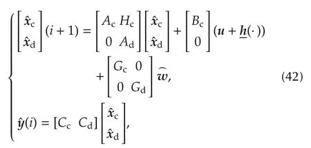
where initial conditions and timeihave been omitted,the inline vector notation of[11]allows us to writethe sub-matrices,the nonlinear termand the initial state are known,and the commanduis the same dispatched to the plant.The state vectorx=[](inline notation)is observable fromandis controllable byu.In the simplest case,is controllable bywhere the inverted breve“⌒′′signifies estimate,and the caret“′′signifies one-step prediction.

Of the four uncertainty classes in[11],namely,causal and parametric uncertainty,initial state and neglected dynamics,(42)only retains thecausal uncertaintyexpressed by.The other three classes are expressed with the help of thedesign model,which surrogates the plantPof Section 2.3.The design model output isy(the plant output)and the state is the vectorx=[xc,xd],which is the homologous ofxin(42)and plays the role of thetrue state.Theparametric uncertainty,not treated in Section 2.3,is the difference Δh=h(xc)−)with respect to the design-model termh(xc).Theinitial stateuncertaintydefines the initial prediction error.Thefractional error operator∂Pof the neglected dynamics is defined as in(11),by decomposingyas follows:

whereymis the homologous ofin(42)and plays the role of the model output of the design model.Finally,wmis the random measurement error(absent in Section2.3).∂Pis here approximated by a linear operator represented by the transfer matrix∂P(s).Some properties of∂P(s)can be found in[11].The case study in Section 4 will point out an unstable∂P(s)not treated in[11].The input disturbancedin(17)is now a signal of the design model and holds

wherewcis not marked to signify the uncertainty class of the design model.

Separation between parametric uncertainty and neglected dynamics is a design issue as pointed out in[17].As a rule,Δhdoes not add any dynamics to the model,but describes nonlinear terms,cross-coupling and parametric uncertainty to be rejected.On the contrary,∂Paccounts for short-term additional dynamics(delay,resonance,partial differential equations)whose contribution toymust be blocked from spilling into embedded model and control law.This is the goal of thenoise estimator(z)=N(z)(y−)(z),which implies that the feedbackFmof Fig.2 is factorized asFm(z)=D(z)N(z).

IfGcis not full rank(butGdcan be designed to be full rank),two singular cases may occur as in Section 4.

1)State derivatives close to the outputare noise free,like the point-mass velocity(the same applies to the tank level rate in Section 4).In this event,a static output-to-noise feedbackNcannot stabilize the embedded model and must be replaced by a dynamic feedback.However,a staticNmay be employed,if a measurement of the noise-free state derivatives is made available as in navigation problems(see[11]and[18]).

2)State derivatives close to the model commanduare noise free like in Section 4,where the plant command is the integral of model commandu.In this case,the relevant states are stabilized by the control law and not byN.

The design of the sub-matrices{Hc,Gc,Ad,Gd}and ofN,which has been referred to as the noise design in[19],aims to distribute the necessary and sufficient uncertainty input points to the embedded model.The generic state equation ofNis the following:

whereihas been partly omitted.The equation pair that consists of(42)and(45)constitutes astate predictor(SP),which replaces thealmost linear plantof Section2.3.The term state predictor is preferable to state observer since(42)naturally provides the state one-step prediction.The quintuple of matrices{Lc,Ld,Nc,Nd,Ae}must be designed to stabilize the SP complementary spectrum Γm={γmj},with γmj=1 −λmj,j=1,...,nm(pole placement).The sizeneofxedepends on rankGc.

If we assume thath(xc)is unknown(in other terms=0 in(42)),theZ-transform of the output prediction error=y−ymcan be proved as in[11]to satisfy thedesign equation

where the pair{Sm,Vm},which has been already employed in(15)is a function of Γm,mis the model error defined in(11)and(43),anddyis the output disturbance defined in(17).The identity in(46)becomes the first part of the control unit in Fig.6,where the EMC error loop is drawn.

In a more detailed way than the normed inequality(16),(46)distinguishes between two sets of uncertainty contributing to:

Fig.6 The error loop according to embedded model control.

1)The first one is the uncertainty depending onymlike the output of the fractional error∂P(ym)in(43)andh(xc)in(44).Their bounded uncertainty sets∂P(·,p) ∈∂P andh(·,p) ∈H are parameterized by a bounded setp∈Π of parameters.

2)The second one is the uncertainty which is independent ofymlikewmin(43)andHcxd+Gcwcin(44).Their uncertainty sets can be defined by their bounded PSD,(f)ofwmand(f)ofw=[wc,wd],which has been already employed in(41).

3.2 Second design steps:control law and tracking error

As a control performance,the prediction error in(46)must be replaced by thetrue output tracking errorr=r−ym,not to be confused with the classical control errorr−y.The output error is related to the measured tracking errorerof the control law as follows:

Equation(47)assumes the matrix identityCd=CcQ,which is part of the Davison-Francis equation[11]

Equation(48)fixes the disturbance rejection matricesQandPof the control law

whereuris the reference command,which satisfies the controllable dynamics,and the feedback matrixKstabilizes the complementary spectrum Γc={γcj},j=1,...,ncofAc−BcK.

In[11],theZ-transform ofrhas been proved to satisfy a similar equation to(46),namely:

where the pair{S,V}is referred to as theoverall sensitivityandoverall CSas they account for the closedloop plant,Swis referred to as thecausality correctionand the expression of the factors can be found in[11].The namecausality correctionindicates thatSwcannot be zeroed,Sw≠0,since the estimated noiseG(i)withG=[GcQGd],cannot be canceled by the control law(49)because of causality.In fact,under white noise assumption,the noise one-step prediction is zero,i.e.,(i)=0,and the subtraction of a term proportional to(i−1)in(49)just increases the tracking error covariance.Since in practice,due to inaccurate rejection,(i)may include residual correlated components,they may be further attenuated by adding to(49)a stable dynamic feedback directly driven by(y−y)(i)[20].The term plays a role similar to Youla parameterization[21].Let us observe that,at first sight,the CSVc(z),which played a role in Section 2.3,does not appear in the last row of(50).Actually,we can prove thatVc(z)=c(z),and beingVc(0)=I(low-pass filter),the frequency BWfcofVccan be defined.

In[11],Swhas been proved to be a band-pass transfer matrix,which makes the bandwidths{fs,fv}of{S,V}narrower than the BWs{fms,fmv}of{Sm,Vm}.Fig.7(a),clearly shows the phenomenon.Narrowing the sensitivity BW is detrimental to the tracking error accuracy(“bad effect”)since the unknown disturbance rejection is band-limited.Narrowing the CS BW may be of benefit(“good effect”)as it makes the state predictor more effective in blocking the contribution of the neglected dynamics to the control law.Equation(50)and the role ofSwlook an advancement of the theory in Section 2.3,and are reflected by the last part of the error-loop blockdiagram of Fig.6.

The design implications of the new error loop in Fig.6 can be better appreciated by extracting,frommin(43)anddyin(44)(in practice fromh),the uncertain components which depend onymand hence on the tracking error,and therefore are prone to destabilize the closed loop plant.Following[11],we rewrite(50)as

where the argumentzhas been partly omitted,Dy(z)transfers the noise vectorwontoy,and∂H(z)is computed by assuming thath(xc)is a sector-bounded nonlinearity.

Closed-loop stability can be ensured by fixing the worst-case elements ∂Pworst(z)= ∂P(z,pworst)and∂Hworst(z)= ∂H(z,pworst)of the uncertainty sets,and by applying either the Nyquist criterion or the small gain theorem to the loop functionV(z)∂Pworst(z) −S(z)∂Hworst(z).Small-gain theorem allows the argument uncertainty to be ignored.

If σmax(∂Pworst(jf))and σmax(∂Hworst(jf))dominate the high-and low-frequency bands of 0≤f＜fmax,respectively,the small-gain inequality can be split into the pair of inequalities

where the norms in(52)are defined by ‖E(jf)‖∞=The frequency domain separation in(52)can be further exploited by approximatingV(z)andS(z)with their HF and LF asymptotesV∞(z,Γ)andS0(z,Γ),respectively,as they are analytically related to the elements of Γ.Moreover,since the result of a pole placement which satisfies(52)is the frequency BW pair{fs(ηs),fv(ηv)},which is constrained byfs(ηs)＜fv(ηv)＜fmax,failure of the latter inequality indicates that pole placement cannot ensure closed-loop stability versus the given uncertainty.

Given a feasible η =max?ηs,ηv?＜1 and,for simplicity’s sake,by assuming zero reference,i.e.,r=0,(51)can be transformed into the pair of performance inequalities

where+=1,the frequency domain has been separated,{Sw,Sd}denotes the spectral density bounds ofwmanddy,andSy,maxis the spectral bound of the output tracking error which is allocated to the pair of inequalities in(52)through the weight pair{ws,wv}.Stability and performance inequalities in(52)and(53)can be combined into a single functional to be minimized below unity.Moreover,performance inequalities can be converted into variance inequalities,which are equivalent to the weighted norm in(20).

The above inequalities are expressed in terms of{S(Γ),V(Γ)},but which is the interplay with the SP pair{Sm(Γm),Vm(Γm)}of the first design step?Letbe the frequency BW pair of the state predictor(SP).Two pole placement strategies have been pointed out in[11].

1)Thestandard designguarantees that the SP sensitivity is not degraded bySw,which amounts to satisfy the frequency inequality

wherefcis the frequency BW ofVc.The inequality implies and is implied by ‖Sw‖∞＜ 1,and in turn implies that the norm of the measured tracking error|r−|tends to be a numerical zero,smaller than the output quantization,a condition that can be in-field verified.

2)Thenonstandard designaims tofc＜fmvand impliesfs＜fms,with the consequence that the SP sensitivity is degraded as in Fig.7(a).The design becomes mandatory to account for command saturation and for avoiding saturation instability.The case study of Section 4 will adopt this strategy,since “crude”command saturation is allowed between two successive set points.

4 Case study

The EMC design steps in Section 3 are now applied to a well-known multivariate control problem.

4.1 From tank dynamics to the design model

Consider the four-tank control problem in[13];the layout is sketched in Fig.8.

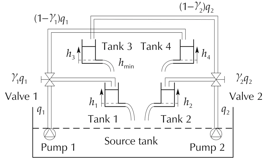
Fig.8 Sketch of the four-tank layout.

Two pairs of cascaded tanks{k=1,3}and{k=2,4}are fed by two pumps denoted by the subscript{j=1,2}.The pair of lower tanks{k=1,2}discharges into the common source tank and are fed by one of the upper tanks and by one of the pumps with the rule:{j=1,k=3}→k=1 and{j=2,k=4}→k=2.The pair of upper tanks{k=3,4}is just fed by the pumps with the reverse rule of the lower tanks,i.e.,j=1→k=4 andj=2→k=3.The pump flows are distributed to tanks by regulating the valves 1 and 2 to the fractions 0≤γ1≤1 and 0≤γ2≤1.The fractions are collected in the vector γ =[γ1,γ2](inline vector notation).Thekth tank levelxkis bounded by 0≤xk,min≤xk≤xk,maxand is an entry of the vector 0≤x≤xmax.The level squar?e rootdefines the tank discharge rate,whereSkis the horizontal section area,αkis the discharge constant in m2and g is the local gravity.The pump flow rate 0 ≤qk=φk/Sk(m ·s−1)≤qk,maxis collected in the vectorqand depends on the pump command vector[φ1,φ2](m3·s−1).

The nonlinear fourth-order state equation(see[22])is written,without initial conditions,as

where 0≤x≤xmax,0≤q(t)≤qmax,τuis a transport delay,τyis the level sensor delay,yis the tank level measurement corrupted bym,qdcollects the flow perturbations due to leakage and model inaccuracy,and the following notations apply:

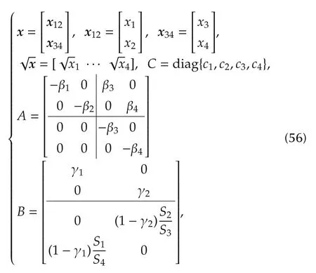
whereBcan also be written asB=[B12B34].In(56),qmaxis the pump maximum flow andck=1+sk,sk≪1 being the scale factor error.As soon asx→0,the measurement errormbecomes biased by the least measured level denoted byxmin＞0.The limit will be employed by the control unit to boundxfrom below,when necessary.

The control goal is to force the lower-tank levels inx12to track the referencer12=[r1,r2],where,as in[22],the reference profile is a sequence of set points,which are equilibrium points of(55).Given the equilibrium vectorsatisfying the limits in(56),the command and upper tank equilibrium valuesare given by

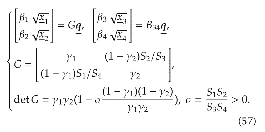
The zero determinant detG=0 distinguishes two regulation problems.

1)Direct lower tank regulationfor detG＞0.The corresponding inequality(1/γ1−1)(1/γ2−1)＜ 1/σ implies the valve fraction direction γ → [1,1]and the convergence to detG=1.Under this condition(see Fig.8),the lower tanks can be directly and independently regulated to the set point,which must satisfy the pump flow and upper tank limits.The lower tank dynamics is just first order.The upper tank dynamics,under the lower tank regulation,plays the role of a zero dynamics[14],which is locally asymptotically stable.The corresponding discharge flow is treated as a disturbance.

2)Indirect lower tank regulationfor detG＜0.The corresponding inequality(1/γ1−1)(1/γ2−1)＞ 1/σ implies the valve fraction direction γ → [0,0],and the convergence to detG= −σ.Under this condition(see Fig.8),the lower tanks must be regulated through the upper tanks and the input-output relative degree becomes two.In fact,for detG= −σ,as proven in[22]and[23],the upper tank dynamics,under direct lower tank regulation,becomes a locally unstable zero dynamics[14]and the upper tank levels tend to saturate.Unlike in[23],where a combination of the lower and tank levels was regulated([22]showed that a mixed regulation cannot regulate the lower tanks in the presence of unknown disturbances),Section 4.2 and the following will show that the indirect regulation cannot just be addressed by converting(55)into the normal form of the feedback linearization[14],since the resulting normal form happens to be driven by the derivative of the pump flow,and the relevant extended dynamics[14]is nonlinear,uncertain and affected by a non-collocated disturbance.Moreover,since any disturbance flow affecting the lower tanks will be accommodated by the varying level and discharge rate of the upper tanks,level set-points must be carefully selected.

The indirect regulation has been approached in[24]by the sliding model control in the region 0.1 ≤ γ1,γ2≤0.2.Here,the first step is to derive a CT design model via feedback linearization and extended dynamics(Section 4.2).A LTI design model is the basis for building the stabilizing ideal control law in Section 4.3.The same model is the source of the DT embedded model(57)in Section 4.4.In the same Section,the model is stabilized by a dynamic noise estimator of the same kind as in equation(45)and the ideal control law is converted into its real form.Section 4.5 is devoted to the pole placement in the presence of causal uncertainty(random flows),parametric uncertainty and neglected dynamics.The design inequalities of Section 3.2 will be employed.A nonstandard pole placement is adopted to cope with ’crude’pump-flow saturation during set-point switching.Section 4.6 will illustrate and discuss simulated results in the fraction region 0 ≤ γ1,γ2＜0.5,to check the previous design in the presence of uncertainty.

4.2 The design model

In view of the indirect regulation,we transform the fourth-order equation(55)into a non-minimum-phase sixth-order equation with zero eigenvalues and one positive transmission zero.Let us define the controllable statexcthrough a smooth transformationf(x),x＞0,and the inclusion of the pump flow rateq:

where initial conditions have been omitted,d=[d1,d2]is the unknown disturbance,h(·)is a cross-coupling term,and the following notations apply:

The pair of variable transmission zeros holds

The state-dependent matrixG34(xc)can be confined into the command matrix,but the state-feedback design does not change,since the relative degree does not change from two to three and a normal form cannot be obtained.

Fig.9 shows the block diagram of(59).Delays are represented by blocks with an inscribed D.A double-border box denotes a nonlinear function.The variable gainpkis denoted with an arrowed circle.Vertical arrows denote initial conditions.The parametersbk,k=1,...,4,are the nonzero entries of the matrixBin(56),the subscriptkbeing the row index ofB.

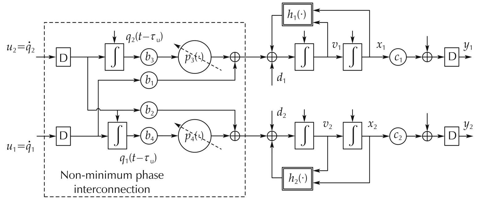
Fig.9 Block diagram of the design model.

4.3 Ideal control law

Let us neglect the command delay τu(to be part of neglected dynamics),and includeh(·)(assumed to be unknown)intod.Let the tracking error of the lower tanks be written as(the set point)is a sequence of equilibrium points in(57)satisfying tank and pump bounds.Similarly,we define the level rate error12r=v12and the flow rate error=q−qr+Q(x)d,whereqr=has been defined in(57),andQtestifies thatdis not collocated.The ideal stabilizing control law of(59)is given by

where the identityKx=Kx(xc)applies to the three gain matrices,which depend onxcthroughG34(xc).Because of the bound|xc|≤xc,max,which derives from the boundedxandqin(56),G34(xc)＞0 is bounded from below and from above and the feedback gains in(62)can be designed by assuming that the nominal matricesare symmetric and constant during a set-point interval of the reference profilexr(t)=[x12r,x34r].The matrix discrepancy

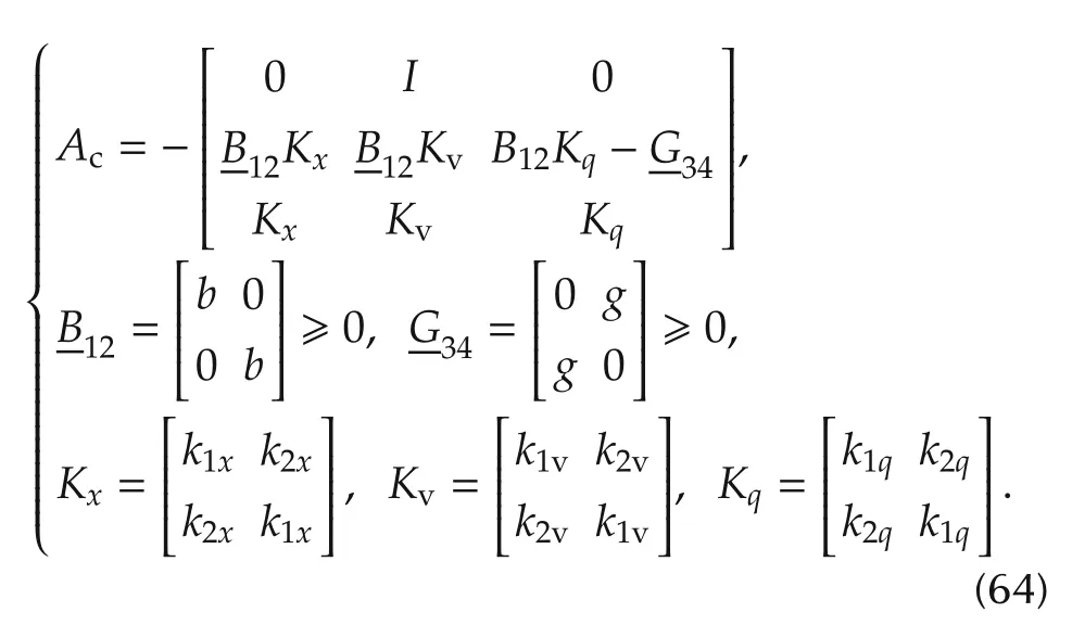
Because of the aforementioned symmetry,the characteristic polynomial Π(Ac,λ)can be factored into a pair of third-order polynomials,whose coefficients are related to the sub-matrix entries in(64).Given a Hurwitz spectrum Λc= Λ(Ac)and the coefficients in

the gains in(64)are found by solving an algebraic equation,which admits a unique solution forb==＜1 in the matrixcan be found from the Davison-Francis equation(48),if applied to the embedded model of Section 4.4.

4.4 Embedded model and real control law

The next step amounts to convert(59)into a DT embedded model like that in equation(42).The model must include the disturbance dynamics and must provide the one-step prediction of the command beforeti+1=(i+1)T.The real control law generates the plant command as the digitized pump flownqand the flow rate derivative in(62)as a function of the measured tracking errors as follows:

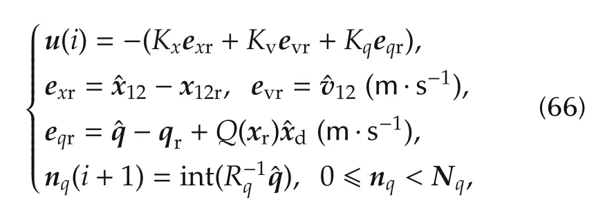
where the timeihas been partly omitted,the last row expresses command digitization and saturation,nq(i)andNqare integer vectors andRqholds:

wherek=1,2.

The embedded model aims to one-step predicting the controllable stateand the unknown disturbance(i)(in acceleration units).The possible improvement of the one-step prediction in(66)by the current measurementy(i)is not considered.The pair of decoupled fourth-order equations,in the form of(42),is as follows:

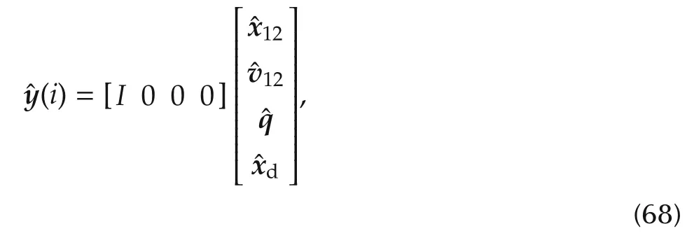
where timeihas been partly omitted,the unknown disturbance is the sum of the noise(including the command quantization error)andof the first-order random driftdriven by the noise.In practice,the three equations of(59)are completed with that of.Transport and sensor delays are confined into the neglected dynamics.Parametric errors come from the uncertainty ofB12and the uncertainty and time variability ofG34.

The matrixGcof(42)that multiplies is singular,since no component is driving the first and third rows of(68).The zero first row implies that a dynamic noise estimatorHmust be adopted,as in[11]and in equation(45)in order to stabilize the embedded model.In this case,only four diagonal matrices{Ae,Lc,Nc,Nd}are necessary and sufficient to stabilize the pair of fourth order state predictors,which consists of(68),without the third row,and of(45)withLd=0.The one-to-one relation between the AS spectrum Λm={Λmk,k=1,2}with Λmk={λmkj,j=1,...,4},|λmkj|＜ 1,and the eight gains of the diagonal feedback matrices{Ae,Lc,Nc,Nd}is straightforward(see[11]).

4.5 Pole placement

The assignment of the complementary spectra Γc(control law)and Γm(SP),which possess a total of 7+7 eigenvalues,is driven by two objectives.The first one isasymptotic stabilityin the presence of uncertainty and pump flow saturation.The second is theaccuracyof the lower tank level around the required set points in the presence of random flows,measurement errors and parametric uncertainty.We assume that the nominal valve fractions are uniform and equal,i.e.,

4.5.1 Stability

We do not adopt a reference generator that minimizes the tracking error during set-point switching.This implies“crude”saturation of pump flows and instability because of the relative degree＞1.According to EMC design[11],command saturation can be managed by adopting the non-standard design of Section 3.2(an alternative solution is to shape the feedback gains as satu-rating functions).In essence,we adoptfc(Γc)＜fmv(Γm)wherefcrefers toVc(Γc)andfmvtoVm(Γm).In terms of the real complementary eigenvalues γcj()∈ Γc,j=1,...,6 and γmj∈Γm,j=1,...,8,we impose the inequalities

Following[11],the eigenvalues are spread with the following rules

where{αc≥ 0,αm≥ 0}is a second pair of tunable parameters.

Given(70),{αc,αm}have been tuned for guaranteeing closed-loop stability versus neglected dynamics due to delays and the parametric uncertainty ΔG34(xc)+in(63).To be simple,we only focus on the fractional error∂Pin(51),by including ΔG34(xc)in ∂P.The effect ofas a component of∂Hwill not be studied.The design inequality to be adopted is just the first row in(52).

In order to build up∂P,we treatG34(xc)andP12(xc)as perturbed constant matrices,which allows us to writeP(s)appearing in the transfer relationx12(s)=P(s)q(s)(design model)as follows:

where τ = τq+ τy≤ 2 s is the unknown total delay andP12is a bounded unknown.The zero-order interpolated transfer matrix in(s)=M(s)q(s)(embedded model)holds

wherez=exp(sT)withs=j2πf,and the second-row approximation applies forf＜π/T.

The open-loop fractional error∂P(s)=P(s)M−1(s)−Iturns out to be unstable,since one of the transmission zeros ofM(s)is real positive as pointed out by(61).However,the closed-loopV(s)∂P(s)is internally stable,since the transmission zeros ofV(s)include those ofM(s),and thus cancel the poles ofM−1(s).We have to guarantee stability in the presence of the worstcase ∂Pworst(s),which corresponds either toG34,max=G34(x34r,min)or toG34,min=G34(x34r,max)depending on(xr).The resulting pair{αc,αm}is reported in Table1.

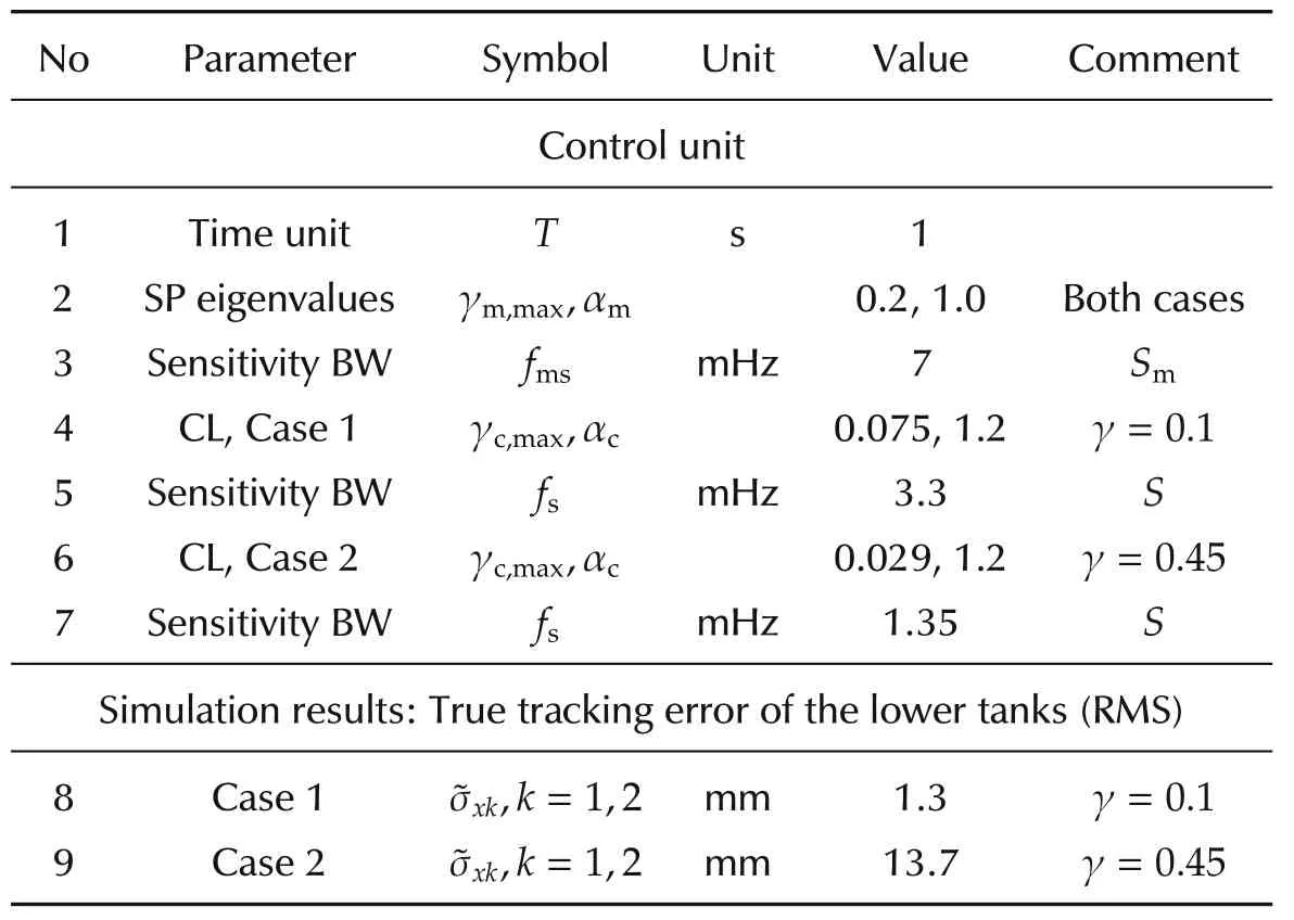
Table 1 Control unit parameters and simulation results.

As a check,the Nyquist plot of det(I+∂Pworst(jω))−1(the open-loop case)and of det(I+V(jω)∂Pworst(jω))−1(the closed-loop case)are shown in Fig.10,for=0.1(simulated Case 1,Fig.10(a)),for=0.45(simulated Case 2,Fig.10(b))and for the pairSinceV(s)∂Pworst(s)has no unstable poles,both Nyquist plots ensure closed-loop stability as they do not encircle the critical point(−1,0).

Fig.10 Nyquist plot of the open loop and closed-loop fractional error for the pair{G34,min,G34,max}.The large closed curve corresponds to the open-loop case.(a)Case1.(b)Case 2.

4.5.2 Accuracy

“Crude”saturation suggests that accuracy requirement only concerns steady state level fluctuations and the transient time duration τjsince the switching timetrj.The accuracy indicator is the a posteriori RMS‖xk=xk−xkr‖of the tracking error,which is defined by

forNjT≤tr,j+1−(trj+τj).Given the pole placement in(69)and(70),accuracy can only be predicted from the inequalities in(53).The first one is concerned with the measurement noise,whose contribution can be proved,in the present simulated case,to be less significant than the random flowqdin(55).Thus,we restrict the analysis to the second inequality,whereis the spectral bound,in length units,of the random flow componentsqd1,k=1,2(m·s−1)contributing to the lower tank level.

SinceSd(f),in order to be bounded-variance,must be bounded and decreasing forf＞fd,σmax(S(jf,Γ)Sd(f))turns out to be band-pass.By assuming thatfdandfshave the same order of magnitude,we expect that mfa x σmax(S(jf,Γ)Sd(f))occurs in the same frequency region.Fig.7(a)showsthat,for=0.1(but the same expression applies to any),the sensitivity low-frequency asymptote holds:

Therefore,if the decreasing profile ofSdforf＞fdis approximated as follows(parameter values are in Table2):

where κ ＞1 is a conservative factor andfSD＞fsis an estimation of the spectral density bandwidth.Fig.7(b)compares the computed boundand the simu-lated RMS‖xk‖versus the nominal≤0.49.Since the computed RMS tracks the simulated RMS,it is employed to fix the boundwheren=3,to the steady-state tracking error.

Table 2 Simulation parameters.

for α＞1.

4.6 Simulated results

Simulation parameters are reported in Table2.The nominal value of the uncertain parameters to be used in control design and implementation are reported together with their maximum uncertainty(in percent).

Control unit parameters and results are reported in Table1.We distinguish between the SP sensitivitySmand the overall sensitivityS.DT complementary eigenvalues γk=1−λkare reported together with the relevant frequency BW.

The tracking error RMS in Table1 has been computed by neglecting the transient profile between two successive set points and the zero set-point intervals.Fig.11 shows the time history of the lower and the upper tank levels for γ=0.1(Case1).Whereas lower-tank levels accurately track their set points(true-level and set-point cannot be distinguished in Fig.11(a)),upper-tank levels fluctuate around their set points to allow compensation of random flows and of set-point switching transients.The level peaks indicate the latter compensation.

Fig.12(a),shows,for the Case 1,the pump commanded flows and the relevant set points.Pump flows are biased because of the parameter perturbations in Table2,which confirms the efficient role of the random driftdof(68)in predicting and rejecting random flows and parameter perturbations.Pump flows saturate without significant oscillations,which confirms the CL eigenvalue design in equation(70).

Fig.12(b),compares the true tracking error1=x1−x1r(solid line)and the measured tracking error e1r=1−x1r(dashed line)of the tank 1.Due to a nonstandard design,these errors are different only during the zero set-point intervals t=[0,5)ks and t＞50ks.For t＞50ks,except during the set-point switching interval,the true tracking error,though biased,is close to zero,sincex1→x1r=0.Instead−x1→y1,min=20mm,i.e.,it equals the least sensor measurement(see Table2,row 6).Fort＜5ks,both tracking errors should tend to fluctuate around zero sincex1→y1,min.However,since the upper tank levels saturate down to zero(see Fig.11(b)),they become incapable of compensating the lower-tank random flows.As a result,1→0,whereasx1diverges from zero.

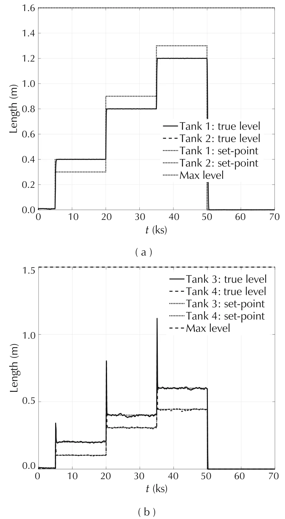
Fig.11 Case 1.(a)Lower-tank levels.(b)Upper-tank levels.

Fig.13(b),shows the tracking errors of the Case 2.The same considerations as for the Case 1 apply,except that one of the upper-tank level remains close to zero fort∈[5,20)ks(Fig.13(a))and impedes the regulation of the tank 1 level.Fort＞20ks,the tracking errors increase as predicted by Fig.7(b),but,outside the transient intervals,they stay within the target bound.

Fig.12 Case 1.(a)Pump flow.(b)Tank 1 tracking errors.

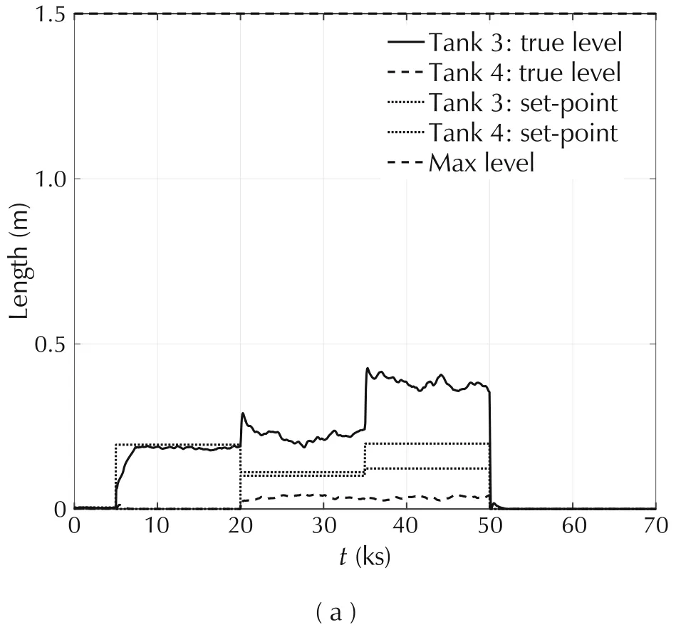
Fig.13 Case 2.(a)Upper tank levels.(b)Tank 1 tracking errors.

As a conclusion,simulation results fit the accuracy requirements expressed by equation(77)and Fig.7(b).

5 Conclusions

The goal and effort of the paper was in the line of reconciling the modern control theory of[2]with the error-based design principle of the centenary PID of[5],still the work-horse of the closed-loop control systems in any application field.To this end,we have recalled in some detail the robust control theory of[10]with the aim of pointing out the concept and equations of the error loop,whose stability has been proved to be necessary and sufficient for the real plant stability.The forward path of the error loop is the cascade of the uncertain discrepancies between plant and model in series with the transfer functions of the modern control theory.The input signals of the error loop are reference signals and the bounded arbitrary(hence unpredictable)signals of the R.Kalman’s theory(white noise process in the stochastic framework).The uncertain discrepancies are assumed to belong to parameterized sets,which,being bounded,imply that reality may generate incompatible outliers.The relevant detection and the consequent control system reconfiguration is outside of the paper scope.Error loop equations are converted by the embedded model control into design inequalities(similar to those of the H-infinity design methods),where control transfer functions are parameterized by the closed-loop eigenvalues to be designed(pole placement)versus stability/performance requirements and worst–case uncertainty.Frequency domain decomposition and transferfunction asymptotes allow the designer to find analytic inequalities capable of providing first-trial closed-loop poles and their margin versus stability and accuracy.The method is applied to a well-known multivariate control problem,which does not admit the feedback linearization normal form.

6 Acknowledgments

The authors are grateful to Prof.Z.Gao,Cleveland State University,Cleveland,Ohio,for his precious indications and suggestions.