The impact of spatial autocorrelation on CPUE standardization between two different fi sheries*

XU Luoliang (许骆良) 2 CHEN Xinjun (陈新军) 2 GUAN Wenjiang (官文江) 2 TIAN Siquan (田思泉) 2 CHEN Yong (陈勇)

1College of Marine Sciences,Shanghai Ocean University,Shanghai 201306,China

2Key Laboratory of Sustainable Exploitation of Oceanic Fisheries Resources(Shanghai Ocean University),Ministry of Education,Shanghai 201306,China

3National Engineering Research Center for oceanic Fisheries,Shanghai Ocean University,Shanghai 201306,China

4School of Marine Sciences,University of Maine,Orono,ME 04469,USA

AbstractCatch per unit of effort (CPUE) data can display spatial autocorrelation. However, most of the CPUE standardization methods developed so far assumes independency of observations for the dependent variable, which is often invalid. In this study, we collected data of two fi sheries, squid jigging fishery and mackerel trawl fishery. We used standard generalized linear model (GLM) and spatial GLMs to compare the impact of spatial autocorrelation on CPUE standardization for different fi sheries. We found that spatial-GLMs perform better than standard-GLM for both fi sheries. The overestimation of precision of CPUE estimates was observed in both fi sheries. Moran’s I was used to quantify the level of autocorrelation for the two fi sheries. The results show that autocorrelation in mackerel trawl fishery was much stronger than that in squid jigging fishery. According to the results of this paper, we highly recommend to account for spatial autocorrelation when using GLM to standardize CPUE data derived from commercial fi sheries.

Keyword:spatial autocorrelation; catch per unit effort (CPUE) standardization; squid jigging fishery;mackerel trawl fishery

1　INTRODUCTION

Catch per unit effort (CPUE) is often used as an index of abundance in stock assessment models(Harley et al., 2001; Campbell, 2004). However,nominal CPUE could be affected by many variables including spatial-temporal factors or environmental factors in addition to stock size. The assumed proportionality between observed CPUE and stock abundance could be shifted by these factors. CPUE standardization, which involves statistical analyses to remove the effects of other variables and extract the year trend of stock abundance, has become a routine in fishery stock assessment (Tian et al., 2009;Campbell, 2015). Many statistical methods have been used to achieve this goal as for example generalized linear model (GLM), generalized additive model(GAM), regression tree and generalized linear mixed model(GLMM) (Guan et al., 2014). Of all these methods, GLM is most commonly used (Dunn, 2009;Li et al., 2015; Walsh and Brodziak, 2015).

GLM is a fl exible generalization of ordinary linear regression. Three basic assumptions need to be fulfi lled when using GLM. Firstly, each of the dependent variables should follow a particular distribution from the exponential family such as normal distribution, poisson distribution, binomial distribution and gamma distribution. Secondly, the relationship between the link function of expected values of dependent variables and independent variables is linear. Thirdly, each elements of the dependent variables is observed independently(Nelder and Wedderburn, 1972). Violation of these assumptions may invalid CPUE standardization results, reducing the quality of the data used in stock assessment.

The third assumption is not always true in fi sheries due to fi sh aggregation and movement, and behavior of fi sherman (Nishida and Chen, 2004). CPUE data are often fishery-dependent, and therefore observations may not be independent and are likely to be spatially correlated.

Several studies have been conducted to compare the performance of different methods and models used to standardize CPUE indices (Hinton and Maunder, 2004). However, spatial autocorrelation is not as apparent as other problems in CPUE standardization, such as the presence of null catches or collinearity in the independent variables.Incorporating spatial autocorrelation is not yet generally perceived to be a requirement in CPUE standardization. Untill recently attention has been given to the spatial autocorrelation problem in CPUE standardization (Yu et al., 2011; Thorson et al., 2015;Jiao et al., 2016) though majority of studies dealing with CPUE standardization do not account for spatial autocorrelation.

Ecologists have been aware of spatial autocorrelation for a long time and methods for handling it have been used in other fi elds (Dormann,2007). Subsampling was one of the approaches used to avoid spatial autocorrelation by keeping removing observations that are too close together until residual spatial autocorrelation is low or negligible. However,this method is far from optimal and the “imperfect information” is better than “no information”.Researchers also tended to struggle with the idea of removing hard-collected data. In addition to subsampling, other statistical methods to explicitly model spatial autocorrelation are available (Cressie,1993). The basic theory is that in regression models,if the data are truly independent, the variance around the expected value is modelled as Var(x)=σ2/(n-1),whereσ2is the population variance andn-1 is the degrees of freedom. For spatially autocorrelated data,this variance gets an additional component, which specifi es the covariance between values ofxat locationsiandj(Haining, 2003; Dormann, 2007):

It is obvious that in a spatially autocorrelated context, true variance should be larger than the variance resulting from non-spatial model as the term Cov(xi,xj) is always positive. Therefore, ignoring spatial autocorrelation can lead to variance underestimation.

However, some ecologists argue that spatial autocorrelation contains information that one might not want to “correct for” and spatial autocorrelation in data results from environmental factors as well as ecological factors. Thus, we need to include as independent variable all the key factors to be able to model the process responsible for spatial autocorrelation. If spatial autocorrelation is observed in the residuals of the model, it may result from the model lacking one or several key factors (Guisan and Thuiller, 2005; Dormann, 2007 ). On the other hand,others argue that the so called ‘correct’ independent variables are not easy or even impossible to be observed at the required resolution or at the necessary biological accuracy (Dormann, 2007). In fact,statistical models such as GLM or GAM are not population dynamic models, they can hardly model real ecological processes even if the model includes all significant factors.

CPUE standardization is not the same as modeling species distribution, although they use the same statistical models and they have the same spatial autocorrelation problem. The simple purpose of CPUE standardization is to extract the year trend of stock abundance to be included in the assessment models but not to explain why the stock is abundant or to predict species distribution. Nishida and Chen(2004) fi rstly introduced a statistic method called spatial-GLM into CPUE standardization to account for spatial autocorrelation, which was used for yellowfi n tuna caught in longline. In this study, we applied spatial-GLM to standardize CPUE of two important oversea fi sheries in China, squid jigging fishery and mackerel trawl fishery, and we evaluated the impact of spatial autocorrelation on the CPUE standardization results.

2　MATERIAL AND METHOD

2.1　Data source

We obtained data from Chinese Distant-water Fishery Association for jigging fishery for jumbo squid (Dosidicusgigas) and trawl fishery for Chilean jack mackerel (Trachurusmurphyi) in high seas of Southeast Pacific (Fig.1). The logbook information included data on daily catch (t), fi shing effort (days fi shed), fi shing dates (year, month, day) and locations(longitude and latitude). The spatial and temporal resolutions of fishery data were 0.5°×0.5° and month respectively. The nominal CPUE in the fi shing unit of 0.5°×0.5° was calculated as follows:

where CPUEymijwas nominal CPUE ,CymijandFymijwere the sum of catch and the sum of fi shing effort,respectively, at longitudei, latitudejin monthmand yeary.

The time series range from 2003 to 2012 for squid jigging fishery and from 2002 to 2011 for mackerel trawl fishery. We chose sea surface height (SSH, the height of the ocean’s surface which are often affected by ocean circulation), sea surface temperature (SST)and chlorophyll-aconcentration (CHL) as environment variables in the CPUE standardization because these variables were shown to be critically important in inf l uencing distribution of these two species (Li et al., 2016; Yu et al., 2016). The environmental data were downloaded from the National Oceanic and Atmospheric Administration(NOAA) at http://oceanwatch.pifsc.noaa.gov/las/servlets/dataset. All the environmental variables were averaged by 0.5°×0.5° for each month to match the spatial-temporal resolution of fishery data.

2.2　Standard-GLM

The term standard-GLM, was used to refer to standard GLM to distinguish it from the spatial-GLM.For both fi sheries, the CPUE data follow a log-normal distribution. The standard-GLM takes the following form:

where CPUE is the nominal CPUE; θ is a constant,which is set at 10% of the global mean of nominal CPUE (Guan et al., 2014) and added to avoid zero CPUE value;kis the intercept;xiare independent variables including year, month, SST, SSH and CHL;aiare the related coeffcient; andεis the error term,assumed to follow a normal distribution with zero mean and an unknown fi xed standard errorσ. The parameters were estimated by maximum likelihood(ML).

2.3　Spatial-GLM

For the spatial-GLM, Eq.3 above was modified as:

Fig.1　The fi shing grounds of two fi sheries

Unlike standard-GLM, under spatial-GLM, the random errorsεare allowed to have a multivariate normal distribution with zero mean and a variancecovariance matrix denoted byV. The covariance cov(εi,εj) is a function of the distance between locationiandj. To calculate the distancedijbetweenitoj, we used haversine formula which using a great-circle calculates the distance between two points on a sphere from their longitudes and latitudes. The following four equations were used to model the spatialautocorrelation:

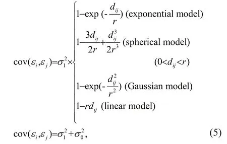
whereσ02is the nugget effect andσ12is the partial sill.The parameters were estimated by the method of restricted maximum likelihood (REML). The loglikelihood function can be defi ned as follows:

Table 1　The comparison of different levels of autocorrelation by Moran’s I

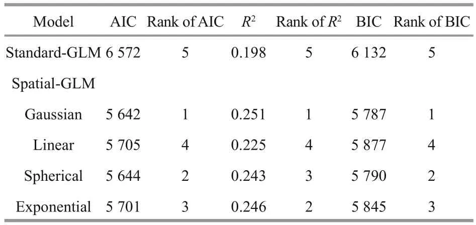
Table 2　Summary of AIC, BIC and R2ranks of each models for squid jigging fishery

2.4　Spatial autocorrelation testing

Before applying spatial autocorrelation on CPUE standardization, we checked if spatial autocorrelation existed in the data. We used Moran’s I to test global spatial autocorrelation (Dormann, 2007). The values of Moran’s I were used to represent the level of spatial autocorrelation for the two fi sheries. Moran’s I is defi ned as:

whereNis the number of spatial units indexed byiandj;Xis the variable ofinterest which corresponds to the CPUE in this study;is the mean ofX; andwijis an element of a matrix of spatial weights (Zhang and Lin, 2008).

2.5　Relative difference of estimate of standardized CPUE

The relative difference of standardized CPUE was evaluated by comparing the estimated CPUE values from standard-GLM with those from spatial-GLM.

whereθ1is the CPUE estimates from standard-GLM andθ2is the CPUE estimates from spatial-GLM.

3　RESULT

3.1　Spatial autocorrelation testing

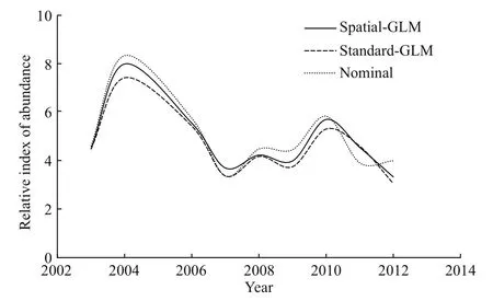
Fig.2　The nominal CPUE and standardized CPUE of squid jigging fishery

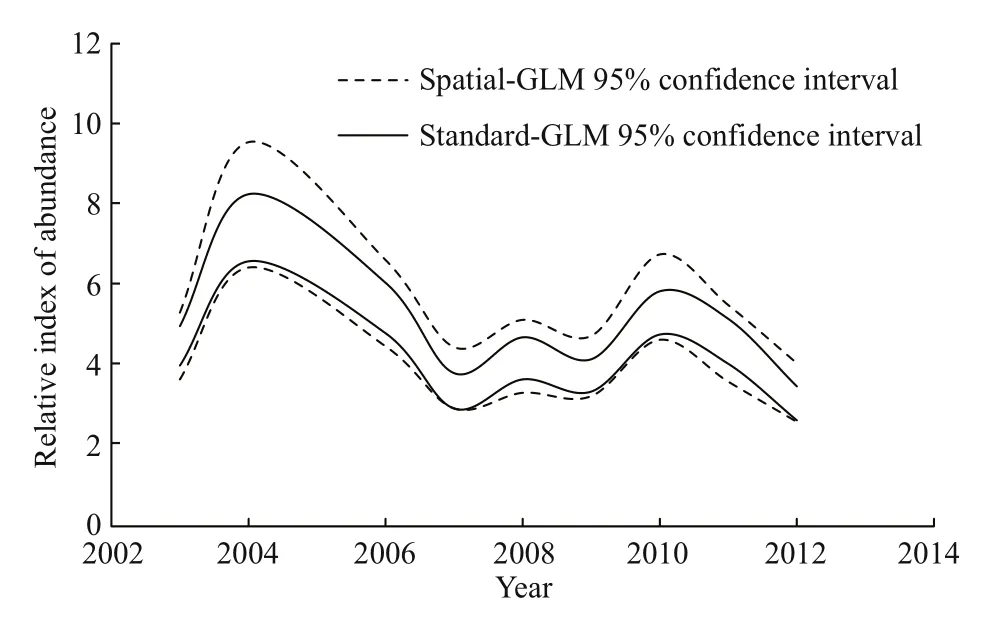
Fig.3　Comparison of 95% confi dence interval of relative abundance index estimate by two models for squid jigging fishery

Based on theP-value (P＜0.05), we reject the null hypothesis that there is no spatial autocorrelation in CPUE (Table 1). In both cases, Moran’s I was positive,which means that the spatial autocorrelation is positive.Moran’s I was higher in mackerel trawl fishery than in squid jigging fishery (Table 1) suggesting that spatial autocorrelation was stronger in the mackerel trawl fishery than in the squid jigging fishery.

3.2　Standard-GLM vs spatial-GLM for squid jigging fishery

According to the AIC and BIC (Table 2), we concluded that all spatial-GLMs fi tted better than the standard-GLM and Gaussian distance spatial-GLM model fi tted the data best for the squid jigging fishery.R2increased from 0.198 for the standard-GLM to 0.251 for the Gaussian distance spatial-GLM in squid jigging fishery.

Therefore, Gaussian distance spatial-GLM model was chosen as the fi nal model to compare with the standard-GLM model.R2increased from 0.234 for the standard-GLM to 0.319 for the exponential distance spatial-GLM. The temporal trends in CPUE did not differ greatly from each other (Fig.2). However, the range of the 95% confi dence intervals of the spatial-GLM is larger than that of the standard-GLM (Fig.3).

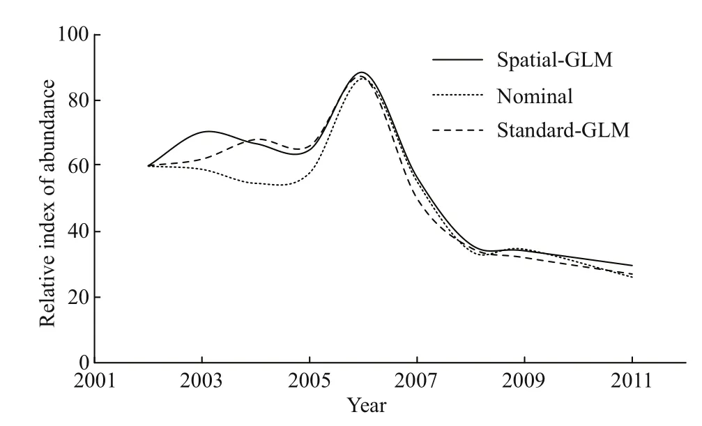
Fig.4　The nominal CPUE and standardized CPUE of mackerel trawl fishery

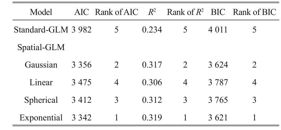
Table 3　Summary of AIC, BIC and R2ranks of each models for mackerel trawl fishery

3.3　Standard-GLM vs spatial-GLM for mackerel trawl fishery

According to the AIC and BIC (Table 3), all the spatial-GLMs fi tted better than the standard-GLM and the exponential distance spatial-GLM fi tted the data best. We therefore compared the results of the exponential distance spatial-GLM model with the results of the standard-GLM model.

The temporal trends of nominal CPUE and standardized CPUE by the two different models do not differ greatly from each other. However, the relative difference of CPUE estimates is high in some years (Table 5). The range of the 95% confi dence intervals of the spatial-GLM is larger than that of standard-GLM (Figs.4, 5).

3.4　Relative difference of standardized CPUE and level of spatial autocorrelation

The relationship between relative difference of standardized CPUE and corresponding level of spatial autocorrelation was tested by Pearson correlation test. In both fi sheries, the relation was significantly positive. In squid jigging fishery, the Pearson correlation coeffcient was 0.67 (t=2.412 5, df=7,P=0.047). In mackerel trawl fishery, the Pearson correlation coeffcient was 0.71(t=2.631 9, df=7,P=0.034) (Table 5).

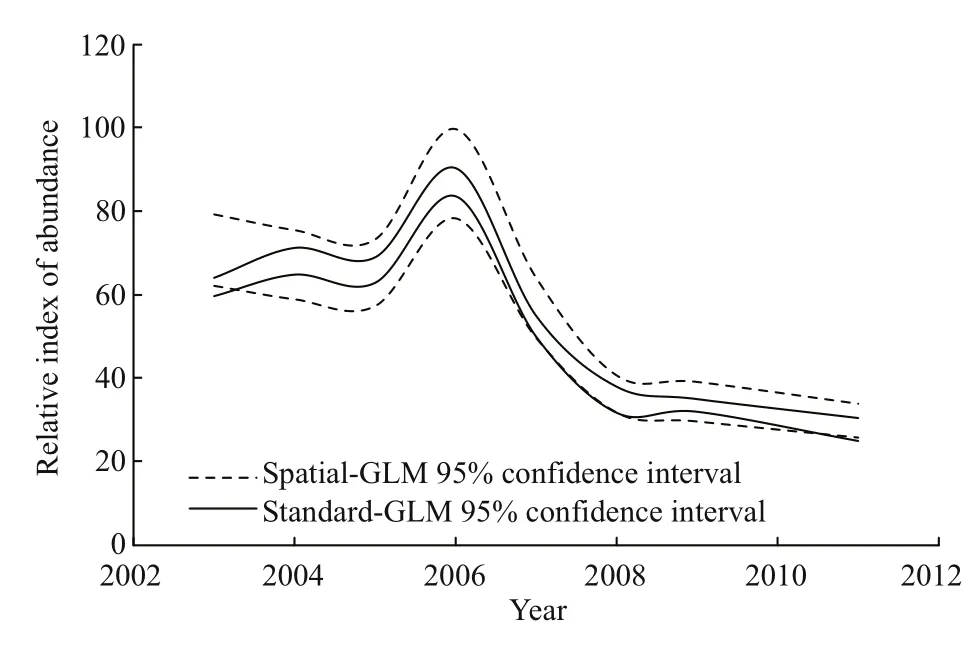
Fig.5　Comparison of 95% confi dence interval of relative abundance index estimate by two models for mackerel trawl fishery

4　DISCUSSION

4.1　Overestimation of precision by standard-GLM and better-fi tting by spatial-GLM

In general, the temporal trends of CPUE standardized by standard-GLM and spatial-GLM did not differ greatly, but yearly estimates of relative abundance index differed (Table 5, Figs.2, 4). Also,the relative difference of standardized CPUE was correlated to the level of spatial autocorrelation,which indicated that for a given year with higher spatial autocorrelation the estimate of standardized CPUE differed greater. The difference in the estimated temporal variation of the abundance index might affect stock assessment results.

When the standard deviation and 95% confi dence intervals estimated by two models were compared, an overestimation of precision in the standard-GLM for both fi sheries was evident. This might be a general problem when spatial autocorrelation is not accounted in CPUE standardization, which was shown also in tuna long-line fishery by Nishida and Chen (2004).This is mainly because spatial autocorrelation in CPUE observations increases effective sample size but do not provide suffcient independent information.This problem was described as “pseudo replication”by Carl and Kühn (2007) described this problem as“pseudo replication”where the real number of degrees of freedom is lower than the one used in the standard-GLM. Thus, the standard-GLM underestimates the real uncertainty of the CPUE estimates in standardizing CPUE. Because the inverse value of variance is often used as a weighting factor for a time series of CPUE in stock assessment, the overly optimistic standard errors may result in unnecessarily large weight for the CPUEs estimated from the standard-GLM.

Species distribution models with or without consideration of spatial autocorrelation for plants,invertebrates, birds, mammals and herpetofauna were compared by Dormann (2007). The results showed that coeffcient estimates in all cases were affected by spatial autocorrelation, leading to a bias of 25% on average. Only one of 20 spatial models performed worse than its standard model, but the meanR2value of models incorporating spatial autocorrelation increased to 0.49 from 0.43. In the fi sheries considered here, the relative difference associated to the estimates of CPUE was not severe. The relative difference associated to the estimates of CPUE from two models was related to the level of spatial autocorrelation as quantified by Moran’s I (Table 5). Based onR2, AIC and BIC, we conclude that the spatial-GLMs performed better in analyzing CPUE data for both fi sheries used in this study.

4.2　The level of spatial autocorrelation in different fishery

In species distribution models, there are both exogenous and endogenous mechanisms to introduce spatial autocorrelation into data (Liebhold et al.,2004). Exogenous factors often include temperature,wind speed, water type or other environmental factors(Dormann, 2007). In some cases, the models including proper exogenous factors display no spatial autocorrelation in residuals (Hawkins and Porter,2003; Bhattarai et al., 2004), which indicates that exogenous factors might be the main reason for species autocorrelation in these cases. The spatial autocorrelation distance (i.e. the maximum distance in which data are interdependent) of pelagic fi sh is correlated to the temperature of depth where the fi sh is distributed. The spatial autocorrelation distance of temperature increases with increasing depth. Due to greater homogeneity of deeper ocean waters, the spatial autocorrelation distance of species living in deeper water will be greater (Kleisner et al., 2010).Compared with well-designed scientific research with random sampling, fi shing vessels always concentrate on the area where the target species is abundant,which may cause systematic bias of CPUE data(Maunder et al., 2006).

Different fi sheries use different gears and fi shing methods. This may be the main reason why level of spatial autocorrelation is different between squid jigging fishery and mackerel trawl fishery. Based on the Maron’s I (Table 1), the spatial autocorrelation in mackerel trawl fishery is much stronger than in the squid jigging fishery, which might result from how the different species are fi shed. The Chinese squid jigging fishery in the Southeast Pacific is a lightattracting fishery. It can only be operated at dark nights. At the daytime after sunrise, the squids cannot any longer be attracted and aggregated by light. They spread out and dive into the deep ocean even through the oxygen minimum zone (OMZ) (Seibel, 2013;Stewart et al., 2013). The daily and seasonal vertical and horizontal migrations are typical behavior forDosiducusgigas. This may lower the spatial autocorrelation in the fishery data. The mackerel trawl fishery operates continuously during day and night. The fi shermen in the industrial vessels are usually divided into 3 groups and take turns to work and rest. In addition, the depths of water which mackerel stays between day and night do not greatly differ. If a high concentration of fi sh is discovered in one Specific location, the fi shermen will operate for several days in the same location. Meanwhile, vessels belong to one fl eet or one company would aggregate in the same location. Because of that, the squid jigging fishery provides more random CPUE data than the mackerel trawl fishery and thus less autocorrelation.

4.3　Exploration of CPUE data derived from fishery

Data quality is extremely important in fishery research (Tian et al., 2013). Fishery-dependent data from logbook are far from perfect. There are routine steps to explore the data before a CPUE standardization, namely, (1) removing the outliers;(2) judging the distribution of CPUE; (3) dealing with zero catch; and (4) testing the collinearity between dependent variables. The independence hypothesis is frequently ignored in CPUE standardization. In fact,depending on fi sheries, the spatial autocorrelation can be substantial (Table 1). At present, no standard approach is developed to explore data under spatial autocorrelation before CPUE standardization. We consider this aspect of any CPUE standardization as important and thus we recommend to evaluate whether there is dependence in the CPUE raw data before any CPUE standardization analysis.

We compared Maron’s I of residual in the standard-GLM and spatial-GLM (Table 4). In both fi sheries,Maron’s I of residual was lower for the spatial-GLM,which indicates that the spatial autocorrelation was reduced in spatial-GLM. However, according to theP-value, the spatial autocorrelation still exists and thus was not totally removed by the spatial-GLM.

Table 4　The Moran’s Index of residue of different models

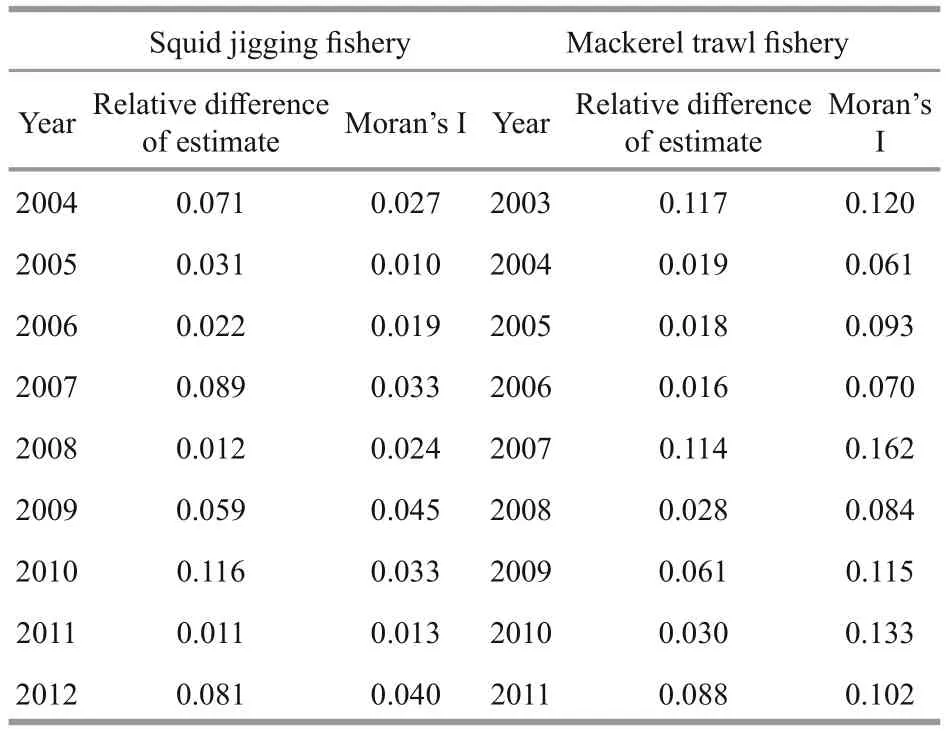
Table 5　The Moran’s I and relative difference of estimate of relative abundance index in each year

4.4　Future research

Temporal and spatial resolutions of data in this study are month and 0.5°×0.5°respectively. This may be appropriate for such time series and at the large scale of the fi shing grounds described here. However,Tian et al. (2013) found that combinations of different spatial and temporal resolutions could have different impacts on the standardization of CPUE. The choice of spatial-temporal resolution used in GLM may add uncertainty in the CPUE estimates. In the spatial-GLM model, different resolutions of data may also inf l uence the results since some detailed spatial information would be omitted at low temporal and spatial resolution. Thus, a study of the impact of different spatial and temporal resolutions would be necessary.

There are two factors that could cause spatial autocorrelation in CPUE data. One of them is fi sh aggregation and movement in relation to environment factors. The other is the concentration of commercial fi shing vessels in the same fi shing area causing nonrandom sampling, which could produce bias in the CPUE standardization process. However, there are no studies that have attempted to separate factors that lead to spatial autocorrelation and evaluate how much the spatial models are actually less biased than standard models. We suggest that using simulated data with controlled spatial autocorrelation is an appropriate approach to verify this hypothesis. In this way, we can compare the estimated parameters by models with or without accounting for spatial autocorrelation with the “true” parameters and observe how the data fi t the models.

5　CONCLUSION

Data derived from logbook of commercial vessels are cheap to acquire. As for large fi sheries as those described here, the fishery-dependent data are informative on the stock biomass trend. Also, when some stock assessment lacks survey data, which is a common case in oversea fi sheries, fishery-dependent data are the only available sources ofinformation for tuning the assessment model. However, fishery dependent CPUE data is of less quality than those derived from standardized scientific surveys.Nevertheless, spatial autocorrelation caused by nonrandom observation is an issue we should always account for when standardizing fishery-dependent CPUE data and we consider spatial-GLM as an appropriate method to deal with this issue.

6　ACKNOWLEDGEMENT

We thank Chinese Oversea Fishery Association(COFA) and NOAA for providing data. We are grateful of CHANG Yongbo in College of Marine Sciences Shanghai Ocean University who has spent much time working in a mackerel trawl vessel and provides the information about the fishery. We also thank the Chinese Distant-water Squid Jigging Technical Group for providing fishery data and information.