The carbon fluxes in different successional stages:modelling the dynamics of tropical montane forests in South Ecuador

Sebastian Paulick,Claudia Dislich,Jürgen Homeier,Rico Fischer*and Andreas Huth,3,4

The carbon fluxes in different successional stages:modelling the dynamics of tropical montane forests in South Ecuador

Sebastian Paulick1,Claudia Dislich1,Jürgen Homeier2,Rico Fischer1*and Andreas Huth1,3,4

Background:Tropical forests play an important role in the global carbon(C)cycle.However,tropical montane forests have been studied less than tropical lowland forests,and their role in carbon storage is not well understood. Montane forests are highly endangered due to logging,land-use and climate change.Our objective was to analyse how the carbon balance changes during forest succession.

Methods:In this study,we used a method to estimate local carbon balances that combined forest inventory data with process-based forest models.We utilised such a forest model to study the carbon balance of a tropical montane forest in South Ecuador,comparing two topographical slope positions(ravines and lower slopes vs upper slopes and ridges).

Results:The simulation results showed that the forest acts as a carbon sink with a maximum net ecosystem exchange (NEE)of 9.3 Mg C∙(ha∙yr)−1during its early successional stage(0–100 years).In the late successional stage,the simulated NEE fluctuated around zero and had a variation of 0.77 Mg C∙(ha∙yr)–1.The simulated variability of the NEE was within the range of the field data.We discovered several forest attributes(e.g.,basal area or the relative amount of pioneer trees)that can serve as predictors for NEE for young forest stands(0–100 years)but not for those in the late successional stage(500–1,000 years).In case of young forest stands these correlations are high,especially between stand basal area and NEE.

Conclusion:In this study,we used an Ecuadorian study site as an example of how to successfully link a forest model with forest inventory data,for estimating stem-diameter distributions,biomass and aboveground net primary productivity.To conclude,this study shows that process-based forest models can be used to investigate the carbon balance of tropical montane forests.With this model it is possible to find hidden relationships between forest attributes and forest carbon fluxes.These relationships promote a better understanding of the role of tropical montane forests in the context of global carbon cycle,which in future will become more relevant to a society under global change.

Forest model,Tropical montane forest,Forest succession,Carbon balance,Forest productivity,FORMIND

Background

Tropical forests play an important role in the global carbon cycle.More than 50%of the carbon stored in aboveground vegetation is assumed to be located in the tropics (Pan et al.2011).Additionally,tropical forests are one of the most productive ecosystems(Bonan 2008).In the global carbon cycle,tropical forests are considered to act as a carbon sink(Houghton et al.2009;Beer et al.2010;IPCC 2013).However,at the local scale,forests act as either sources or sinks,depending upon their successional stage and disturbance state(Luyssaert et al.2008;Morton et al. 2014;Anderson-Teixeira et al.2016;Gatti et al.2014).

Tropical montane forests have been studied less than tropical lowland forests,and their role in carbon storage is not well understood(Spracklen and Righelato 2014); they are highly endangered due to logging,land-use and climate change(Beck et al.2008;Colwell et al.2008). The Tropical Andean forests are considered to be one of the world’s biodiversity hotspots(Brummitt and Lughadha 2003),but they experience one of the highest deforestationrates in South America(1.7%,FAO 2009).For South Ecuador deforestation rates of 2.9%were reported for the period from 1989 to 2008(Tapia-Armijos et al.2015).

Scientific knowledge concerning the dynamics of these ecosystems must be improved to ensure the protection and sustainable management of timber,water and other ecological resources provided by these forests.One method that quantifies the carbon balance of forest ecosystems is the eddy-covariance method,which estimates the net ecosystem exchange(NEE)of carbon.However, in montane areas,the classical eddy-covariance method is difficult to apply because it requires a quasi-flat landscape(Oren et al.2006;Richardson et al.2006;Stoy et al. 2013),which is not the case in a high elevation gradient with pronounced gorges and ridges(Kutsch et al.2008). Therefore,alternative methods are needed to estimate carbon balances.Inventories and field experiments are fundamental,but focus on the site level.Another method uses forest models with the strength on spatial and temporal extrapolation.Forest models in combination with forest inventories offer an alternative approach to estimate and extrapolate carbon fluxes.Additionally,this approach allows to explore correlations between carbon fluxes and other forest attributes(e.g.leaf area index and basal area) and to follow these patterns during forest succession.

Process-based forest growth models such as FORMIND (Köhler and Huth 2004;Fischer et al.2016)simulate recruitment,mortality and tree growth to analyse spatial and temporal forest dynamics.Thereby,such models can improve our understanding of forest ecology(Pacala and Kinzig 2002).The FORMIND model has been applied to various tropical forests(Köhler and Huth 2004;Rüger et al.2007;Dislich et al.2009;Fischer et al.2014),temperate forests(Bohn et al.2014)and even grasslands(Taubert et al.2012).

In this study,we compared the simulated carbon dynamics of two topographically different forest types in Ecuador:(I)lower slope and ravine forest and(II) upper slope and ridge forest.The main questions of our study are:

a)How does the successional stage of a tropical montane forest affect the local carbon balance?

b)Is there a relationship between the simulated structural forest attributes(e.g.,the relative amount of pioneer trees or basal area)and the carbon flux?

Methods

In this section,we present the study site in Ecuador (ridge forest and ravine forest)and the forest model FORMIND.For this study,the model was extended by a carbon balance module and parameterized for the ravine forest.The model parametrization for ravine forest was compared with an already existing parametrization of the ridge forest.

Study area

Our study area is located in the evergreen montane forest of the Reserva Biológica San Francisco(RBSF)(3°58′S,79° 04′W),which is located on the eastern slope of the Andes in southern Ecuador.The reserve covers an elevation gradient from 1,800 to 3,200 m above sea level(a.s.l.),has an average slope of 40°,and harbours four main forest types. These forest types differ in structure and species composition(Homeier et al.2008;Homeier et al.2010).To date, over 300 tree species have been identified in the 1,000 ha area of the RBSF.

At the elevation between 1,900 and 2,100 m a.s.l.,we distinguished between upperslope/ridgeforestand lower slope/ravine forest(Homeier et al.2008).The ravine forest has a lower stem density but a higher basal area and a higher canopy height(20–25 m)than the less species-rich upper slope forest.The dynamics of the upper slope forest have already been investigated using the forest model FORMIND(Dislich et al.2009;Dislich and Huth 2012).Our study focused on the analysis of the lower slope forest(Fig.1).Typical basal area values for this forest type are 30 m2∙ha−1,whereas the overall stem density is approximately 630 trees per hectare(only trees larger than 0.1 m in diameter at breast height(dbh)). For the upper slope forest typical values are 25 m2∙ha−1for basal area and 2,300 individuals per hectare for overall stem density.All inventory plots have no sign of human impact and are therefore assumed to be in an old growth state(Leuschner et al.2013;Werner and Homeier 2015). A detailed description of the forest inventories used for model calibration(lower slope/ravine forest only)can be found in Additional file 1:Appendix A.

To validate our model results,we used additional forest inventories(matrix plots,Werner and Homeier 2015, plus personal communication).The matrix plots cover six 20 m×20 m plots for each of the two forest types (ravine and ridge),wherein every tree larger than 10 cm dbh was measured in the years 2008 and 2009.Trees that died within this time period were excluded.The method of upscaling these plots to 1 ha is discussed in Werner and Homeier(2015)and resulting values are shown in Table 1.Carbon flux estimations from field data(e.g.aboveground net primary productivity ANPP) which were given in units of tons organic dry matter (tODM),were converted into units of mega gram carbon (Mg C)by applying a factor of 0.44(Larcher 2001).

The FORMIND model

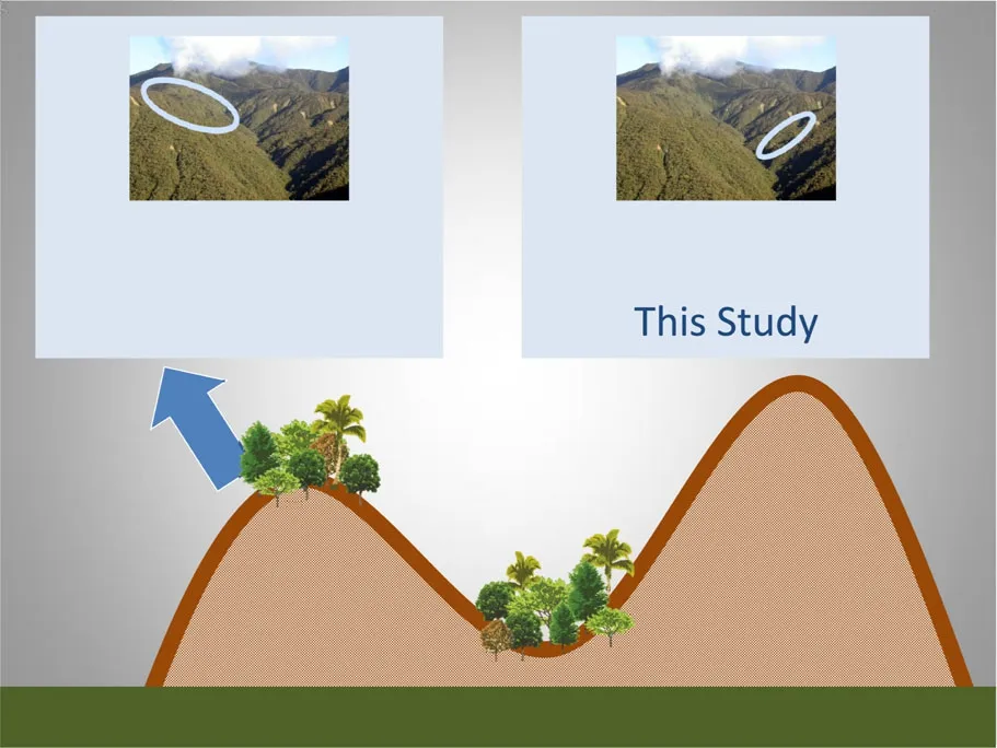
Fig.1 Overview of the study sites in the evergreen montane forest of the Reserva Biológica San Francisco(RBSF).In this study,we focussed on the lower slope/ravine forest and developed a forest model parameterization for this forest type.For comparison,the ridge forest was also investigated(forest model parametrisation taken from Dislich et al.2009,pictures by J.Homeier)

For this study,we utilised the individual and processbased forest gap model FORMIND(Fischer et al.2016). This model is capable of simulating several hundred hectares of forest over a time period of a few centuries. The main processes represented in the model are the establishment of young trees,tree mortality,tree growth and competition for light and space.Tree species within the model are grouped into plant functional types(PFT) according to physiological attributes such as maximum attainable stem diameter and maximum stem diameter growth.All trees within simulation patches of 20 m×20 m compete with one another for light and space.As FORMIND is a process-based model,tree growth is based on a balance between tree photosynthesis and tree respiration rates.For this study,FORMIND was extended by an ecosystem carbon balance module to analyse and estimate all local carbon fluxes between atmosphere,vegetation and soil.

The biomass calculation in FORMIND is based on tree height and diameter at breast height(dbh).Wood density as well as allometric relationships relating tree diameter and height are different for each PFT.The following equation was used to calculate aboveground biomass B (t∙ha−1)for a tree with a stem diameter D(m):

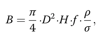
whereby the calculation represents the volume of the tree stem(according to its geometry)multiplied by three factors.Firstly,f[−]denotes a form factor which accounts for deviations of the stem from a cylindrical shape. Secondly,ρ(tODM∙m−3)denotes the wood density and σ(tODM∙tODM−1)represents the fraction of total aboveground biomass included in the stem.The sum of the aboveground biomass of all trees within one hectare represents the biomass of the simulated forest.

For this study,forest dynamics are simulated for 1 ha over a period of 1,000 years using a calculation time step of one year.Each simulation was repeated 10 times(for a total of 10 ha)and was initialised with fallow land. Additionally,we assumed that all carbon stocks in the carbon module are empty(for a description of the different carbon stocks)We differentiated between three successional stages:(a)early succession,from year 0 to 100 years, (b)intermediate succession,from 101 to 500 years,and(c) late succession or old growth stage,from 500 years until the end of the simulation(1,000 years).

In the first step,we analysed static attributes such as basal area,aboveground biomass,stem count,and stem size distribution.In the second step,we analysed advanced and very dynamic forest attributes such as the gross primary production(GPP),aboveground net primary production(ANPP),ecosystem respiration(above-and below-ground)and net ecosystem exchange(NEE).Additionally,vegetation and soil carbon stocks were analysed and compared for both forest types(ravine and ridge forest).It is important to note that all of the carbon pools and carbon flux data presented in this study refer to the projected horizontal area because they pertain to montane forest stands(with an average slope of 33°).

A detailed description of the FORMIND model can be found in Fischer et al.(2016).A list of all model parameters for this study as well as a detailed description of the used carbon cycle submodule is in Additional file 2: Appendix B.1.

The ecosystem carbon cycle module:deadwood and soil-carbon dynamics

In this study,FORMIND was extended by a component to analyse and estimate soil respiration,deadwood respiration and respiration of living biomass.In this module,the model distinguishes between four main carbon stocks:the carbon stored in the living vegetation,deadwood carbon and two types of soil carbon(Fig.2).The deadwood stock contained carbon originating from dead trees,whereas the two soil stocks contained carbon originating from the decomposition of deadwood.The soil separates into two different soil stocks in the different soil layers–one follows a rapid decay process and the other follows a slow decay process(Sato et al.2007).The dynamics of these three stocks are described in the following equations:

?

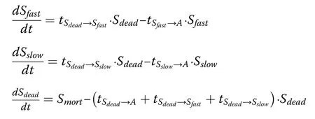
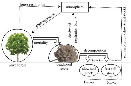
Fig.2 Schematic view of the carbon flux module in FORMIND.Four main carbon stocks were distinguished:the carbon stored in the living vegetation,deadwood carbon and two types of soil carbon. Between all carbon stocks transition rates were calculated(see Additional file 2:Appendix B.2).Each stock has also a respiration flux to the atmosphere.Additionally,carbon from the atmosphere is stored in the forest due to photosynthesis

where CGPPis the sum of the gross primary productivity of all the trees in the forest and CRis the total respiration of all of the living trees in the forest.When the NEE value is positive,the forest takes up carbon.For further details, see Additional file 2:Appendix B.1–B.3 or Fischer et al. (2016).

Parameterisation for tropical montane forest

A full parametrisation of the forest model FORMIND for the ridge forest type has already been developed (Dislich et al.2009).In this study,we parameterised this model for the ravine forest.

The 159 tree species recorded for ravine forest were grouped into nine plant functional types(PFT)(Smith and Shugart 1997;Köhler et al.2000).We used three criteria for the grouping of species:(a)maximum dbh, (b)maximum stem diameter growth and(c)maximum attainable height.Each of these nine PFTs belongs to one of four light demand groups(Table 2).We assumed that light demanding species grow faster than shade tolerant species.There were two fast-growing PFTs(PFT 4 and 8),three medium-fast-growing PFTs(PFT 3,6 and 7),and four slow-growing PFTs(PFT 1,2,5 and 9); subsequently,we will refer to these species groups as pioneer,intermediate and climax species,respectively. A more detailed description of the species groups,including a list of all tree species,is in Additional file 1: Appendix A.5.

For this study,most of the FORMIND model parameter values were determined based on local forest inventories(e.g.,the allometric relationship between dbh and tree height),and some of the parameter values were taken from the literature(see Additional file 2:Appendix B.4).Due to the lack of repeated forest surveys,parameters concerning mortality are unknown.These parameters were estimated using a calibration process that compared the simulated mature forest to the forest inventories.We analysed in detail the total aboveground biomass and the fraction of biomass for each PFT for all trees with a dbh>10 cm.The aboveground biomass ofthe field data was calculated by summing the biomass of the individual trees using the same allometric relationships as used in the FORMIND model(Additional file 2: Appendix B.1).The simulated value for mature biomass was derived by averaging the biomass values of simulated mature forest(year 500–1,000).For the calibration process,we varied the mortality parameter values and compared the stem size distribution and biomass values to the field values.The model itself does not include topography.However,indirectly,topography was incorporated via some parameter values that are affected by topographic conditions(e.g.mortality,productivity).All parameter values are in Additional file 2: Appendix B.4.

Table 2 Plant functional types and their maximum diameter at breast height,maximum diameter increment and maximum height used for species grouping.For each group some exemplary tree species are shown

Differences of ravine and ridge forest

The two forest sites mainly differ in the availability of nutrients in the soil(fewer nutrients in the upper slope/ ridge forest).This leads to a variation in species composition and productivity.To understand how these differences between the upper slope(Dislich et al.2009)and the lower slope(this study)were modeled,the parameter values for the main processes in the forest model were analyzed in detail(see Table 3).Key processes of the forest model are mortality,productivity and regeneration.According to the model parameters,tree mortality is higher in the ridge forest,than in the ravine forest(5.5%vs.2.2%).This makes sense as ridge forests are stronger influenced by wind and weather than the ravine forest.However,the productivity parameter is 20%less in the ridge forest compared to the ravine forest.An explanation could also be the limited availability of soil nutrients in the ridge forest.Regeneration rates are comparable in the parameterisation for both study sites.

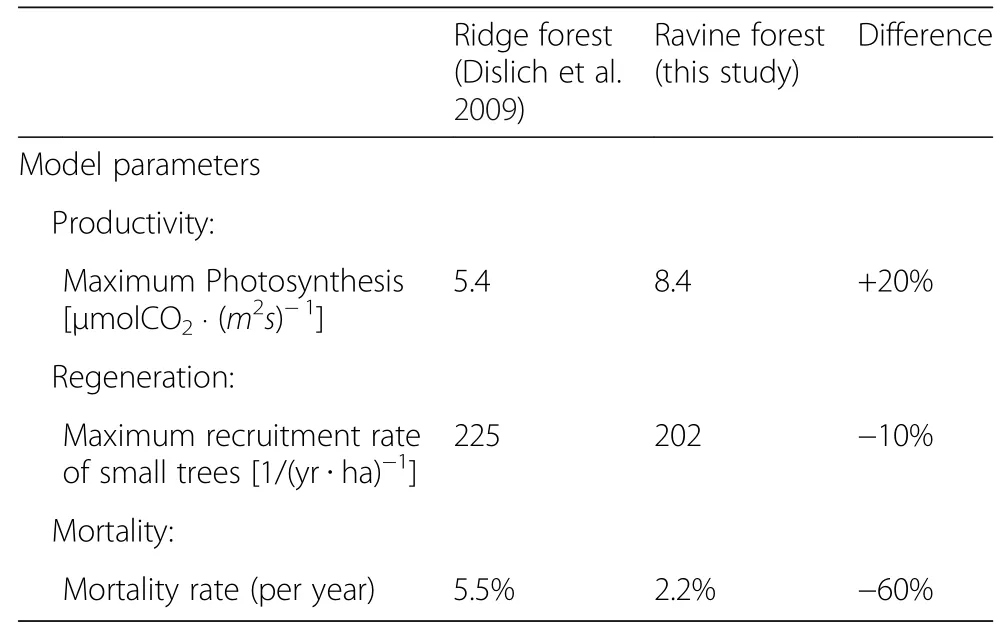
Table 3 Comparison of model parameters for the ridge forest and the ravine forest

Results

The total aboveground biomass of the lower slope ravine forest reached a quasi-equilibrium after approximately 250 years(Fig.3a,221±6.7 tODM∙ha−1),whereas the climax trees did not reach their maximum biomass until after 500 years.During the first 100 years of succession, we observed a high dominance of pioneer trees with biomass values of up to 181 tODM∙ha−1.After 300 years of succession,the tree species with intermediate light demands dominated the forest.After 500 years the species composition more or less stabilised(Fig.3).For the late successional stage,the simulated total aboveground biomass(233.6±11.6 tODM∙ha−1mean over the last 500 years of the simulation)was in good agreement with the field measurements(233.8 tODM∙ha−1).In detail,the biomass of the pioneer species(52.3±17.6 tODM∙ha−1)was in good agreement with field measurements(54 tODM∙ha−1)as well as the biomass of the climax species(45.7±19.4 tODM∙ha−1) comparedtofield data(31tODM∙ha−1).Biomassof intermediate shade tolerant tree species (125.9±18.2 tODM∙ha−1)was slightly underestimated(145 tODM∙ha−1in the field),while the understorey species biomass(11.2±4 tODM∙ha−1)was slightly overestimated(2.6 tODM∙ha−1in the field).The total biomass was in the range of the validation data(271±165 tODM∙ha−1).

In the early successional phase,the forest included many small-sized trees(approximately 425±24.4 per ha, dbh<20 cm),whereas larger trees(dbh>70 cm)were absent(Fig.3b).In the late successional phase(after 500 years),trees attained sizes of up to 110 cm dbh.Also field data and simulation output show a good accordance in the late successional phase(Fig.3c).

The gross primary production(GPP)reached a stable level of approximately 26.3±0.7 Mg C/(ha y)after approximately 350 years(Fig.4a).The aboveground net primary productivity(ANPP)showed a rapid increase within the first 40 years of succession(including a slight overshoot)and then stabilised at values of 3.5±0.5 Mg C/(ha y)(Fig.4a).Within the first 15 years of succession, the net ecosystem exchange(NEE)attained values of up to 9.3±0.06 Mg C∙(ha∙yr)−1(Fig.4b).In later phases,the NEE fluctuated approximately 0.0±0.8 Mg C∙(ha∙yr)−1.

The ridge forest also showed a rapid increase in productivity(GPP and ANPP)during the early successional phase(Fig.4c).After 250 years,the GPP and ANPP reached 25.1±0.6 Mg C∙(ha∙yr)−1and 3.7±0.05 Mg C∙(ha∙yr)−1,respectively,which is on the same order as those for the ravine forest(Fig.4c).In the late successional stage,the NEE of the ridge forest fluctuated approximately 0.0±0.2 Mg C∙(ha∙yr)−1(Fig.4d).

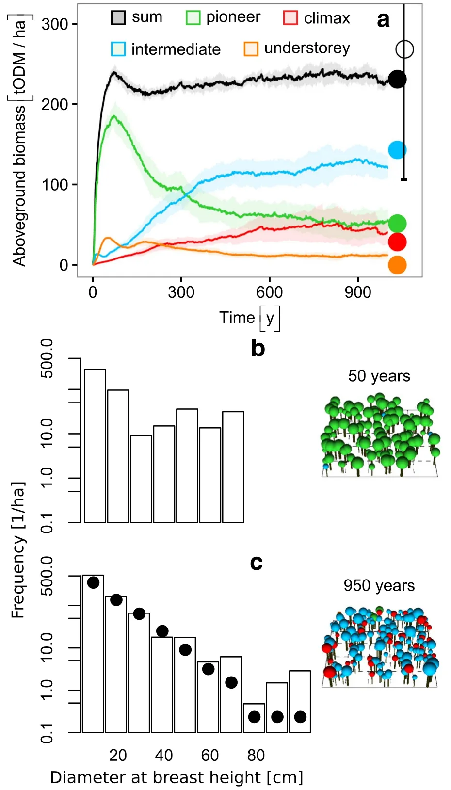
Fig.3 Simulated biomass development and stem size distribution for ravine forest.a Simulated biomass succession over time for the different species groups:pioneers(green),intermediate(blue), understorey(orange)and climax(red).The closed coloured dots represent the field data used for calibration.The black open dot shows the independent validation data from forest inventory plots including all tree groups(Werner and Homeier 2015).The light colours represent the variation between simulation runs(standard deviation for 10 simulation runs of 1 ha).The two graphs below show the stem size distributions for 10 simulation runs of 1 ha for a young forest(b,simulation year 50)and an old-growth forest (c,simulation year 950)and exemplary visualisations(only trees larger 10 cm dbh).The closed black dots represent the field data used for calibration

In addition to analysing forest dynamics,our simulation approach also allowed us to explore the relationships between different forest variables and therefore,provided options for exploring ecosystem relationships which have been explored also in other chronosequence forest studies (Denslow and Guzman 2000;Law et al.2003).In contrast to these field studies,which are based on a few measurements in time,the simulation model allows us to follow patterns across the whole successional phase.In the early successional phase,as long as the fraction of pioneer trees in the forest community was larger than 0.75,we observed two steep gradients in NEE from 0.0 Mg C∙(ha∙yr)−1to 9.3 Mg C∙(ha∙yr)−1in the first 9 years and from 9.3 to 3.4 in the years 9 to 17.As the fraction of pioneer trees dropped from 0.75 to 0.5,we observed NEE values between 3.3 and−0.28 Mg C∙(ha∙yr)−1.In the late successional stage,the relative quantity of pioneer trees and the NEE was relatively stable,with values of approximately 0.24±0.02 and 0.01±0.76 Mg C∙(ha∙yr)−1,respectively. We detected that as the basal area increased during early succession,NEE values increased as well,reaching a maximum value of 9.3 Mg C∙(ha∙yr)−1(Fig.5b,during the first 10 years).After reaching its maximum,NEE experienced a strong decline as basal area further increased.For mature forests,the basal area values were approximately 41.4±0.49 m2∙ha−1and the NEE values were 0.01±0.76 Mg C∙(ha∙yr)−1.

Discussion

The Tropical Andes are a major biodiversity hotspot (Brummitt and Lughadha 2003).To analyse the local carbon cycle of a tropical montane forest,we used the process-based forest model FORMIND.We developed a parameterisation for an undisturbed montane rain forest in the Reserva Biológica San Francisco(RBSF).The simulation results showed a good reproduction of basal area and stem number when compared to field data.The estimated aboveground biomass(233.6±11.6 tODM∙ha−1)for mature ravine forests also agreed well with field values(271.0±165.0 tODM∙ha−1)(Werner and Homeier 2015).

Aboveground forest productivity

Field measurements of gross primary productivity and net primary productivity of tropical montane rain forests are rare.In Table 2,we list some values for tropical montane forests in Peru,which are similar in elevation range to our study site(1,800–2,200 m a.s.l.)(Girardin et al.2010).The Peru sites include some of the dominant tree families that are also present in our study region (Lauraceae and Alzateaceae).The basal area,species number,air temperature(13.5°C–18.0°C)and annual precipitation(1,827–2,472 mm∙yr−1)of the Peru sites are comparable to the sites in Ecuador.In summary,our estimates for the ANPP(3.5±0.45 Mg C∙(ha∙yr)−1),based on combining forest inventories and process-based modelling,are only slightly higher than the field measurements for the forests in the Peru sites(2.5 Mg C∙(ha∙yr)−1) (Table 1).

Fig.5 The net ecosystem exchange(NEE)plotted over(a)the relative quantity of pioneer trees(in terms of stem count)in the forest(PFT 4 and 8)and(b)the basal area of all trees in the forest.Green dots represent the early successional stage(year 0 until year 100)and the black dots represent the late successional stage(year 500 until year 1,000).Results are based on simulation data of the ravine forest,South Ecuador

For the Ecuador sites,some estimates based on field measurements are also available.The field data indicated a difference between the ANPP of ravine and ridge forests(4.6 and 2.9 Mg C∙(ha∙yr)−1,respectively,Fig.4).Our simulations also showed higher ANPP values for the ravine forest(by 8%,0.2 Mg C∙(ha∙yr)−1). trees(number of trees with dbh>10 cm).For the early successional stage,we observed a strong relationship between the relative quantity of pioneer trees (Fig.4a)and the NEE.As the proportion of pioneer trees grew,the NEE increased exponentially.In the late successional stage,no functional relationship was observed.The second attribute we explored is the basal area.Again,there was a strong relationship between the basal area and the NEE in the early successional stage but no signal in the late successional stage.Both of these examples demonstrate that for the early successional stage,proxies can be derived to evaluate the NEE values for a tropical montane forest.

The presented approach has high potential but we also have to acknowledge limitations.Model calibration and validation were done based on the existing field data from mature forest,while important conclusions were derived from model results for different successional stages.A more detailed calibration of the model is possible if we have field measurements from forests at different successionalstages.However, current field data includes also some trees of earlysuccession and mid-succession(due to gap dynamics in the forest).Using this field data(including local scale succession events)and due to the fact that FORMIND is an individual-based model,we have already incorporated tree-related properties for different successional stages.

Conclusion

In summary,we found that(a)process-based forest models in combination with forest inventories are a usefultoolto investigate the carbon balance of tropical forests at a local scale.These techniques allow for the exploration of the dynamics of aboveground biomass and net ecosystem exchange for different successional stages.The different successional stages have a recognisable influence on the forest carbon balance.(b)Additionally,our study explored the relationships between the forest variables and NEE,which appeared to be weaker or stronger depending upon the successional stage of the forest.We discovered a strong signal for the early successional stage but no signal for the late successional stage.These relationships promote a better understanding of the role of tropical montane forests in the context of global carbon cycle.

Additional files

Additional file 1:Field data and model calibration.(PDF 716 kb)

Additional file 2:FORMIND model parameter description.(PDF 194 kb)

Abbreviations

a.s.l.:Above sea level;AET:Actual evapotranspiration;ANPP:Aboveground net primary production;Ca:Carbon;dbh:Diameter at breast height; GPP:Gross primary production;NEE:Net ecosystem exchange;PFT:Plant functional type;RBSF:Reserva Biológica San Francisco;todm:Tons organic dry matter

Acknowledgements

We thank Sven Günter,Patrick Hildebrand and Johana Munoz for collecting field data and establishing the forest plots.The first author would like to thank Franziska Taubert for her comments on this manuscript.The authors also want to thank the anonymous reviewers for their valuable comments. SP,RF and AH were supported by the Helmholtz-Alliance Remote Sensing and Earth System Dynamics.

Funding

We gratefully acknowledge the financial support of the German Research Foundation(DFG,Research Unit 816)for initializing the forest plots and the plot census as well as a first model parameterisation.We also gratefully acknowledge the Helmholtz Alliance:Remote Sensing and Earth System Dynamics for financing the work on the further parameterisation of the model and analysis of the data.

Availability of data and materials

The dataset supporting the conclusions of this article is available through the DFG,Research Unit 816(http://www.tropicalmountainforest.org/).The Software used for modelling is FORMIND(http://www.formind.org).It is platform independent and programmed in C++.It is free to use.

Authors’contributions

SP and AH developed the concept of the paper.SP refined the model parameterisation and did the analysis of the data and adapted the methods used.CD worked on parts of the forest inventory and did a first model parameterisation.JH established most of the used forest plots and acquired the necessary site data for parameterisation.RF also worked on the parameterisation of the model.SP,AH,RF worked on the text.All authors read and approved the final manuscript.

Authors’information

SP studied Applied Mathematics at the University of Applied Sciences in Leipzig,Germany.Now,SP is Ph.D.student at the department for Ecological Modelling at the Helmholtz Centre for Environmental Research–UFZ in Leipzig focussing on montane rain forests.CD has a Ph.D.in Ecological Modelling and is now working at Helmholtz Centre for Environmental Research–UFZ.JH has a Ph.D.in Ecology and is now senior lecturer for Plant ecology and ecosystems research at the Georg-August-University of Göttingen.RF has a Ph.D.in Ecological Modelling and is currently Postdoc at the department for Ecological Modelling at the Helmholtz Centre for Environmental Research–UFZ in Leipzig,focussing on forest modelling and remote sensing.AH has a Ph.D.in Ecological Modelling and has a professorship for Ecological Modelling at the University of Osnabrück.AH is currently also iDiv member for biodiversity modelling at the German Centre for Integrative Biodiversity Research(iDiv)in Leipzig.AH is leading a workgroup for forest modelling at the department for Ecological modelling at the Helmholtz Centre for Environmental Research–UFZ focussing on ecosystem and forest modelling as well as remote sensing. AH is scientific coordinator at the Helmholtz Alliance:Remote Sensing and Earth System Dynamics.

Competing interests

The authors declare that they have no competing interests.

Consent for publication

Not applicable.

Ethics approval and consent to participate

Not applicable.

Author details

1Department of Ecological Modelling,Helmholtz Centre for Environmental Research–UFZ,Permoserstr,15,04318 Leipzig,Germany.2Georg-August-University Göttingen,Plant Ecology,Untere Karspüle 2,37073 Göttingen,Germany.3University of Osnabrück,Institute of Environmental Systems Research,Barbarastr,12,49076 Osnabrück,Germany.4iDiv,German Centre for Integrative Biodiversity Research(iDiv)Halle-Jena-Leipzig, Deutscher Platz 5e,04103 Leipzig,Germany.

Anderson-Teixeira KJ,Wang MMH,McGarvey JC,LeBauer DS(2016)Carbon dynamics of mature and regrowth tropical forests derived from a pantropical database(TropForC-db).Glob Chang Biol 22:1690–1709

Beck E,Bendix J,Kottke I,Makeschin F,Mosandl R,editors(2008)Gradients in a tropical mountain ecosystem of Ecuador.Ecological Studies Vol.198.Berlin,Springer,525 p.

Beer C,Reichstein M,Tomerelli E,Ciais P,Jung M,Carvalhais N,Rödenbeck C, Arain MA,Baldocchi D,Bonan GB,Bondeau A,Cescatti A,Lasslop G,Lindroth A, Lomas M,Luyssaert S,Margolis H,Oleson KW,Roupsard O,Veenedaal E,Viovy N, Williams C,Woodward FI,Papale D(2010)Terrestrial gross carbon dioxide uptake: global distribution and covariation with climate.Science 329:834–838

Bohn FJ,Frank K,Huth A(2014)Of climate and its resulting tree growth: Simulating the productivity of temperate forests.Ecol Model 278:9–17

Bonan GB(2008)Forests and climate change:Forcings,feedbacks,and the climate benefits of forests.Science 320:1444–1449

Brummitt N,Lughadha EN(2003)Biodiversity:Where’s hot and where’s not. Conserv Biol 17:1442–1448

Chave J,Andalo C,Brown S,Cairns MA,Chambers JQ,Eamus D,Folster H, Fromard F,Higuchi N,Kira T,Lescure JP,Nelson BW,Ogawa H,Puig H,Riera B, Yamakura T(2005)Tree allometry and improved estimation of carbon stocks and balance in tropical forests.Oecologia 145:87–99

Chave J,Réjou-Méchain M,Búrquez A,Chidumayo E,Colgan MS,Delitti WBC, Duque A,Eid T,Fearnside PM,Goodman RC,Henry M,Martínez-Yrizar A, Mugasha WA,Muller-Landau HC,Mencuccini M,Nelson BW,Ngomanda A, Nogueira EM,Ortiz-Malavassi E,Pélissier R,Ploton P,Ryan CM,Saldarriaga JG, Vieilledent G(2014)Improved allometric models to estimate the aboveground biomass of tropical trees.Global Change Biol 20:3177–3190

Colwell RK,Brehm G,Cardelus CL,Gilman AC,Longino JT(2008)Global warming, elevational range shifts,and lowland biotic attrition in the wet tropics. Science 322:258–261

Denslow JS,Guzman S(2000)Variation in stand structure,light and seedling abundance across a tropical moist forest chronosequence,Panama.J Veg Sci 11:201–212

Dislich C,Huth A(2012)Modelling the impact of shallow landslides on forest structure in tropical montane forests.Ecol Model 239:40–53

Dislich C,Günter S,Homeier J,Schröder B,Huth A(2009)Simulating forest dynamics of a tropical montane forest in South Ecuador.Erdkunde 63:347–364

FAO,2009.State of the World's Forests 2009.Food and Agriculture Organization of the United Nations(FAO),Rome,p 168.

Fischer R,Armstrong A,Shugart HH,Huth A(2014)Simulating the impacts of reduced rainfall on carbon stocks and net ecosystem exchange in a tropical forest.Environ Model Software 52:200–206

Fischer R,Bohn F,Dantas de Paula M,Dislich C,Groeneveld J,Gutiérrez AG, Kazmierczak M,Knapp N,Lehmann S,Paulick S,Pütz S,Rödig E,Taubert F, Köhler P,Huth A(2016)Lessons learned from applying a forest gap model to understand ecosystem and carbon dynamics of complex tropical forests. Ecol Model 326:124–133

Gatti LV,Gloor M,Miller JB,Doughty CE,Malhi Y,Domingues LG,Basso LS, Martinewski A,Correia CSC,Borges VF,Freitas S,Braz R,Anderson LO,Rocha H, Grace J,Phillips OL,Lloyd J(2014)Drought sensitivity of Amazonian carbon balance revealed by atmospheric measurements.Nature 506:76–80

Girardin CAJ,Malhi Y,Aragão LEOC,Mamani M,Huaraca Huasco W,Durand L, Feeley KJ,Rapp J,Silva-Espejo JE,Silman M,Salinas N,Whittaker RJ(2010)Net primary productivity allocation and cycling of carbon along a tropical forest elevational transect in the Peruvian Andes.Glob Chang Biol 16:3176–3192

Homeier J,Werner FA,Gradstein SR,Breckle S-W,Richter M(2008)Potential vegetation and floristic composition of Andean forests in South Ecuador, with a focus on the RBSF.In:Beck E,Bendix J,Kottke I,Makeschin F,Mosandl R (eds)Gradients in a tropical mountain ecosystem of Ecuador,vol 10.1, 198th edn.Springer,Berlin Heidelberg,pp 87–100

Homeier J,Breckle SW,Günter S,Rollenbeck RT,Leuschner C(2010)Tree diversity, forest structure and productivity along altitudinal and topographical gradients in a species-rich Ecuadorian montane rain forest.Biotropica 42:140–148

Houghton RA,F Hall,and SJ Goetz(2009)Importance of biomass in the global carbon cycle,J.Geophys.Res.,114,G00E03.doi:10.1029/2009JG000935.

IPCC(2013)Climate change 2013:the physical science basis.Cambridge University Press,Cambridge

Köhler P,Huth A(2004)Simulating growth dynamics in a South-East Asian rainforest threatened by recruitment shortage and tree harvesting. Clim Change 67:95–117

Köhler P,Huth A(2010)Towards ground-truthing of spaceborne estimates of above-ground life biomass and leaf area index in tropical rain forests. Biogeosciences 7:2531–2543

Köhler P,Ditzer T,Huth A(2000)Concepts for the aggregation of tropical tree species into functional types and the application on Sabah’s dipterocarp lowland rain forests.J Trop Ecol 16:591–602

Kutsch WL,Kolle O,Rebmann C,Knohl A,Ziegler W,Schulze ED(2008)Advection and resulting CO2exchange uncertainty in a tall forest in central Germany. Ecol Appl 18:1391–1405

Larcher W(2001)Ökophysiologie der Pflanzen.neubearb.Aufl,6th edn.Ulmer, Stuttgart,p 408

Law R,Murrell DJ,Dieckmann U(2003)Population growth in space and time: Spatial logistic equations.Ecology 84:252–262

Leuschner C,Zach A,Moser G,Homeier J,Graefe S,Hertel D,Wittich B,Soethe N, Iost S,Röderstein M,Horna V,Wolf K(2013)The carbon balance of tropical mountain forests along an altitudinal transect.In:Bendix J,Beck J,Bräuning A,Makeschin F,Mosandl R,Scheu S,Wilcke W(eds)Ecosystem services, biodiversity and environmental change in a tropical mountain ecosystem of South Ecuador,vol 10,221st edn.Springer,Berlin Heidelberg,pp 117–139

Luyssaert S,Schulze ED,Borner A,Knohl A,Hessenmoller D,Law BE,Ciais P, Grace J(2008)Old-growth forests as global carbon sinks.Nature 455:213–215

Malhi Y,Aragão LEOC,Metcalfe DB,Paiva R,Quesada CA,Almeida S,Anderson L, Brando P,Chambers JQ,da Costa ACL,Hutyra LR,Oliveira P,Patiño S,Pyle EH,Robertson AL,Teixeira LM(2009)Comprehensive assessment of carbon productivity,allocation and storage in three Amazonian forests.Glob Chang Biol 15:1255–1274

Morton DC,Nagol J,Carabajal CC,Rosette J,Palace M,Cook BD,Vermote EF, Harding DJ,North PRJ(2014)Amazon forests maintain consistent canopy structure and greenness during the dry season.Nature 506:221–224

Oren R,Hseih CI,Stoy P,Albertson J,McCarthy HR,Harrell P,Katul GG(2006) Estimating the uncertainty in annual net ecosystem carbon exchange: spatial variation in turbulent fluxes and sampling errors in eddy-covariance measurements.Glob Chang Biol 12:883–896

Pacala S,Kinzig AP(2002)Introduction to theory and the common ecosystem model.In:Kinzig AP,Pacala S,Tilman GD(eds)The functional consequences of biodiversity:empirical progress and theoretical extensions,vol 8.,pp 169–174

Pan YD,Birdsey RA,Fang JY,Houghton R,Kauppi PE,Kurz WA,Phillips OL, Shvidenko A,Lewis SL,Canadell JG,Ciais P,Jackson RB,Pacala SW,McGuire AD,Piao SL,Rautiainen A,Sitch S,Hayes D(2011)A large and persistent carbon sink in the world’s forests.Science 333:988–993

Richardson AD,Hollinger DY,Burba GG,Davis KJ,Flanagan LB,Katul GG,Munger JW, Ricciuto DM,Stoy PC,Suyker AE,Verma SB,Wofsy SC(2006)A multi-site analysis of random error in tower-based measurements of carbon and energy fluxes. Agric For Meteorol 136:1–18

Rüger N,Gutiérrez AG,Kissling WD,Armesto JJ,Huth A(2007)Ecological impacts of different harvesting scenarios for temperate evergreen rain forest in southern Chile-A simulation experiment.For Ecol Manage 252:52–66

Sato H,Itoh A,Kohyama T(2007)SEIB-DGVM:A new dynamic global vegetation model using a spatially explicit individual-based approach. Ecol Model 200:279–307

Smith TM,Shugart HH(1997)Plant functional types.Cambridge University Press, Cambridge

Spracklen DV,Righelato R(2014)Tropical montane forests are a larger than expected global carbon store.Biogeosciences 11:2741–2754

Stoy PC,Mauder M,Foken T,Marcolla B,Boegh E,Ibrom A,Arain MA,Arneth A, Aurela M,Bernhofer C,Cescatti A,Dellwik E,Duce P,Gianelle D,van Gorsel E, Kiely G,Knohl A,Margolis H,McCaughey H,Merbold L,Montagnani L,Papale D, Reichstein M,Saunders M,Serrano-Ortiz P,Sottocornola M,Spano D,Vaccari F, Varlagin A(2013)A data-driven analysis of energy balance closure across FLUXNET research sites:The role of landscape scale heterogeneity.Agric For Meteorol 171:137–152

Tapia-Armijos MF,Homeier J,Espinosa CI,Leuschner C,de la Cruz M(2015) Deforestation and forest fragmentation in South Ecuador since the 1970s-Losing a hotspot of biodiversity.PLoS One 10:e0133701

Taubert F,Frank K,Huth A(2012)A review of grassland models in the biofuel context.Ecol Model 245:84–93

Werner FA,Homeier J(2015)Is tropical montane forest heterogeneity promoted by a resource-driven feedback cycle?Evidence from nutrient relations, herbivory and litter decomposition along a topographical gradient. Functional Ecology 29:430–440

28 September 2016 Accepted:26 April 2017

*Correspondence:rico.fischer@ufz.de

1Department of Ecological Modelling,Helmholtz Centre for Environmental Research–UFZ,Permoserstr,15,04318 Leipzig,Germany Full list of author information is available at the end of the article

©The Author(s).2017 Open Access This article is distributed under the terms of the Creative Commons Attribution 4.0 International License(http://creativecommons.org/licenses/by/4.0/),which permits unrestricted use,distribution,and reproduction in any medium,provided you give appropriate credit to the original author(s)and the source,provide a link to the Creative Commons license,and indicate if changes were made.