MPM simulations of dam-break floods*

Xuanyu Zhao, Dongfang Liang, Mario Martinelli

1. Department of Engineering, University of Cambridge, Cambridge, UK

2. Deltares, Delft, The Netherlands, E-mail: xz328@cam.ac.uk

MPM simulations of dam-break floods*

Xuanyu Zhao1,2, Dongfang Liang1, Mario Martinelli2

1. Department of Engineering, University of Cambridge, Cambridge, UK

2. Deltares, Delft, The Netherlands, E-mail: xz328@cam.ac.uk

2017,29(3):397-404

Owing to its ability of modelling large deformations and the ease of dealing with moving boundary conditions, the material point method is gaining popularity in geotechnical engineering applications. In this paper, this promising Lagrangian method is applied to hydrodynamic problems to further explore its potential. The collapse of water columns with different initial aspect ratios is simulated by the material point method. In order to test the accuracy and stability of the material point method, simulations are first validated using experimental data and results of mature numerical models. Then, the model is used to ascertain the critical aspect ratio for the widely-used shallow water equations to give satisfactory approximation. From the comparisons between the simulations based on the material point method and the shallow water equations, the critical aspect ratio for the suitable use of the shallow water equations is found to be 1.

Material point method, dam-break floods, Lagrangian method, shallow water equations

Introduction

The material point method (MPM) is an extension of the fluid implicit particle (FLIP) method which was developed from the particle-in-cell (PIC) method to overcome many of its inherent numerical problems in the early implementations. By introducing the Lagrangian particles, the FLIP method eliminates the need to discretise the convective term which is a major source of numerical error in the PIC method[1]. Because of the Lagrangian material description, the FLIP can successfully track material discontinuities and model highly distorted flows[2-4]. The extension of the FLIP method to MPM was originally motivated by the problems of solid mechanics involving history-dependent materials. A distinct feature of the MPM method is that the governing equations are presented in the weak formulation, contrary to the FLIP method. This feature enables the MPM to be consistent with the finite element method (FEM) which has been the dominating computational method in geotechnical engi-neering. Another difference is that the constitutive equations are invoked at the material points in MPM, whereas in FLIP method, they are solved at the fixed grid nodes[3]. Recently, the MPM has been further extended to handle multi-phase problems with a single layer of material points[5-7]or two layers of material points[8-10], and they have been extensively applied to solve engineering problems such as progressive levee failure, pore water pressure development under wave attack on sea dike, seepage flow through embankment, underwater pipeline erosion, etc..

The MPM has many attractive advantages over traditional numerical methods. First, it is convenient to incorporate time-dependent constitutive models because information such as strain, stress, and other timedependent variables can be carried by the moving material points, which enables the spatial and temporal tracking of the history of the material motion. Second, the use of a background mesh allows for the implementation of boundary conditions in a manner similar to the FEM, which is a big advantage compared with other mesh-free methods. In addition, the MPM is free of tensile instability that is evident in smoothed particle hydrodynamics (SPH)[11,12].

In hydrodynamics, free surface hydrodynamics is of significant industrial and environmental importance, but challenges arise in the implementation of surfaceboundary conditions on an arbitrarily moving water surface[13]. Due to the fact that the MPM combines the advantages of the mesh-based method and mesh-free method, it is an attractive method for computing free surface flows. However, despite the above mentioned advantages, there has been little application of the MPM in the field of hydraulic engineering.

Hence, the purpose of this study is to extend the MPM application to free water flow problems and explore the hydrodynamics of the dam-break flows. For the purpose of model validation, the MPM simulations are compared with experimental data and other computational results. Then, a parametric study of the idealised dam-break flow is conducted using the MPM. By comparing its predictions with those based on Shallow Water Equations (SWEs), it is found that the SWEs tend to overestimate the propagation speed of the dam-break flow for initial water columns of large aspect ratios. When aspect ratio of the initial water column is less than 1, then the SWEs give satisfactory predictions. Through these studies, the MPM proves to be a useful tool for investigating hydrodynamic problems.

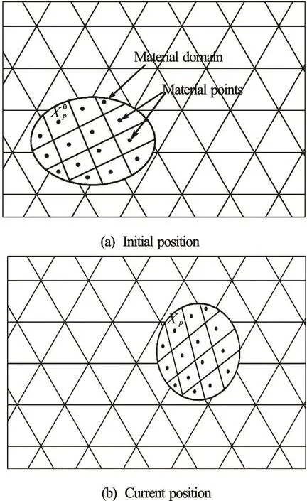
Fig.1 Sketch of background computational grid and the movement of material points

1. MPM model

1.1 Governing equations

Let the material domain W be represented bypN number of material points (Fig.1) and letpxdenote the position of a material point in the current instant (i.e., time t). The same material point in the initial time (t =0) is denoted as.

The governing equations which describe the motion of the continuum body W are the standard conservation equations: mass (Eq.(1)), and momentum (Eq.(2))

where (,)trxis the density of the continuum body, acceleration (,)taxis the material derivative of the velocity, (,)tvxandsis the Cauchy stress tensor that can be decomposed into pressure and deviatoric components. Water pressure is linked to its density change

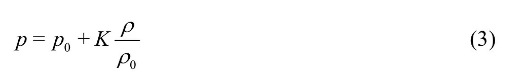
where K is the bulk modulus of water, p is pressure, and the symbols with a subscript indicate the initial reference values.

In the MPM, the non-linear convective term is not present in the formulation as a result of the overall Lagrangian framework[3]. On the contrary, the positions of the material points are updated each time step.

1.2 Weak form of the governing equations

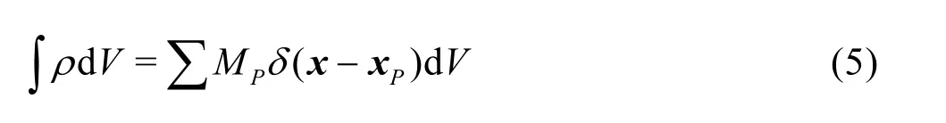
Each material point carries the field variables, mass Mp, density rp(x,t ), velocityvp(x,t) and the Cauchy stresssp(x,t) (p =1,2,3L Np). It is worth noting that the masspM is constant throughout the computation and therefore mass is conserved automatically in MPM. Density of the continuum body at the current instant can be expressed as

where ()d is the Dirac delta function. Then, we have the following relationship

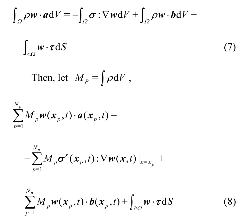
The weak form of the momentum equation can be obtained by multiplying the equation of conservation of momentum by a test functionwas

Applying the divergence theorem in the above equation, the weak form of the momentum equations can be written as

Now considering an Eulerian grid with a total number of nodes Nn, standard nodal basis functions, Ni(x) with i =1- Nncan be defined in the same way as in standard FEM. Then, the variables at the location of a material pointxp, such as the accelerationa(x,t) and the test functionw(xp,t), can be written in terms of nodal basis functions.

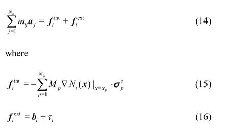
Finally, substituting the relations expressed in Eq.(9) to Eq.(8) results in a discretised equation such that

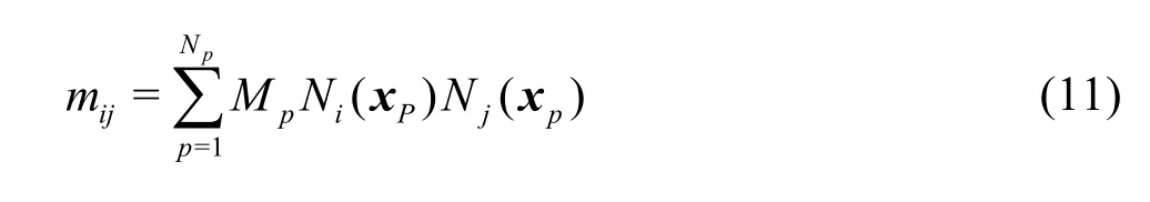
where the mass matrix, mijis defined as

The applied traction,tiis

And the specific body force,biis

Considering the arbitrariness of wi, Eq.(10) can be written in a reduced form, from which the accelerationaat the grid nodes are known by solving Nncoupled linear equations.

1.3 Numerical implementation

In the course of the MPM computation, the unknown variables are always attached to the material points, but they are interpolated onto the grid at the beginning of each time step and their values at the next instant are first computed on the grid. A characteristic of the present implementation is, in order to eliminate divisions by nodal masses, the momentum is used instead of velocity as much as possible in the MPM formulation. Moreover, the velocity gradient used to calculate the strain rate at material points is computed using the updated particle velocities mapped back to the grid nodes[2]. The so-called update-stress-first algorithm is adopted, and the general computational procedure in each time step is as follows. The details of the numerical implementation can be found in literatures[2,3].

(1) Interpolate the mass and momentum from the material points onto the finite element mesh.

(2) Apply boundary conditions on the mesh.

(3) According to the velocities on the nodes, calculate the strain rate and then stress rate at the material points.

(4) Solve Eq.(14) for the acceleration at the nodes of the mesh.

(5) Interpolate the values from the nodes to material points, and then update position of material points.

2. Dam-break problem

It has been common practice to solve shallow water equations (SWEs) numerically for fully dynamic models for flood routing. Shocks in the flow can bereproduced in the form of discontinuities in the weak solution. Being a set of hyperbolic equations, the SWEs admit discontinuities in the solution. They can be derived by integrating the 3-D Navier-Stokes equations over depth, therefore, they are much easier to solve compared with Navier-Stokes equations for the analysis dimension is reduced by one and the free surface position is simply obtained from the mass conservation principle. They are favoured in rapid flood simulations, since for nearly horizontal flows the SWEs description is accurate and convenient.

Due to the space limit, the SWEs model is not quoted here. Detailed discussions of the model are available in many papers. Readers are referred to the papers by Liang[12], Liang et al.[14]and Fraccarollo and Toro[15].

However, Liang[12]questions the accuracy of the results of shock-capturing solver, because he thinks a serious inconsistency behind the shock-capturing schemes to solve the SWEs is overlooked. Close to where the flow changes abruptly, the underlying assumptions behind the SWEs (i.e., hydrostatic pressure distribution, smoothly varied water surface and negligible vertical acceleration) may not hold true. So it may need to evaluate the applicability before solving the SWEs for flood routing. In this section, the MPM model is firstly validated through a dam-break flow problem against the SPH simulation and experimental data. Then, the parametric study of 2-D dam-break flow is conducted using the MPM and SWEs. It should be noted that the MPM model is actually a 3-D model and only one layer of elements are employed to save the computational cost for the width does not actually matter anything.

Fig.2 Sketch of the idealised dam-break problem

It is worth mentioning that in this paper, the name of SWEs instead of a specific solver is used because the aim of this paper is to evaluate the SWEs rather than a specific SWEs solver. The SWEs here are solved by the TVD-MacCormack model which has been extensively verified and applied to many practical case studies[16,17]. As long as different SWEs solvers are correct, their results should be of little discrepancy as they basically solve the same governing equations. Viscous and turbulent effects are not considered in dam-break floods whose behaviours are dominated by convection process. For all the cases in this paper, all the contact surfaces are assumed to be frictionless.

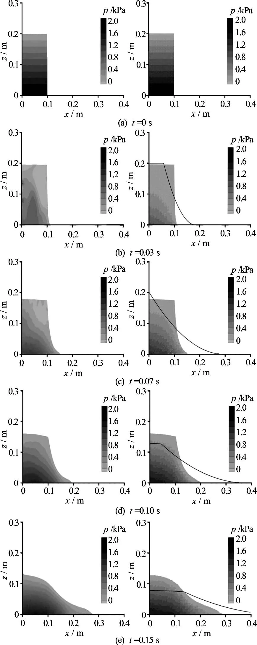
Fig.3 Comparison of the SPH (left) and MPM (right) predictions, with SWEs-predicted water surfaces indicted by solid lines on the MPM plots

2.1 Validation of MPM

In order to validate the MPM algorithm for simulating dam-break flows, the numerical results obtainedfor the dam-break flow with an aspect ratio of 2 are compared with the validated numerical results by SPH presented in Liang[12], where the collapse of a water column onto a horizontal bed is modelled using SPH. The aspect ratio is defined as the ratio of the initial height over the initial width of the water column and is denoted by a. As sketched in Fig.2, a rectangular water column is initially confined between the left wall of the domain and an idealised dam, or vertical wall, on the right. The aspect ratio of the water column is 2.0 with L0=0.1m wide and H0=0.2m high. Once the computation starts, the dam is instantaneously removed and the water is allowed to collapse onto the dry horizontal bed. To achieve a relatively large time step, the bulk modulus of water is assigned an unrealistic low value and this increased compressibility of water does not cause much difference as long as the modelled water has a sound speed over 10 times larger than the maximum flow velocity[12].

The propagation of the flood obtained from the MPM simulation at different time steps are compared with the simulation results using SPH and SWEs models as presented in Liang[12]in Fig.3. The comparison shows a close agreement between the MPM and SPH simulations.

Some quantitative comparisons of the flood front travelling speed are given in Fig.4, where the MPM simulation results are compared against the experimental data[18]and the numerical results obtained using VOF[19], SPH and SWEs solvers[12].

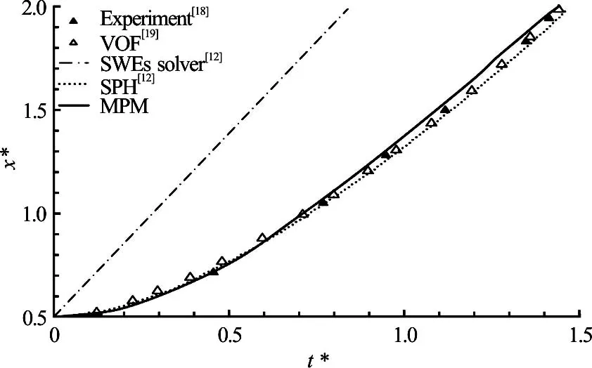
Fig.4 Movement of the flood front position

In order to compare the experimental data of different dimensions, the length and time have been normalised according to the Froude scaling law as expressed in Eq.(17). Here, t*is the normalised time, x*is the normalised flow front position, t is time, x is flow front position,H1height of water column andgis gravitational acceleration.

Generally speaking, the MPM simulations are in good agreement with the experimental data and the numerical results of VOF and SPH. As for the SWEs solver, which assumes negligible vertical momentum, it tends to overestimate the propagation speed of the flood front compared with other methods as a result of the invalid assumption.

2.2 Effect of mesh size and particle density

The dependencies of the dam-break flow simulation on the computational mesh size and particle density (the number of material points per element) are investigated through the simulations of dam-break flow with the aspect ratio of 1. Two mesh sizes are employed: coarse (0.1 m) and fine (0.05 m). Three different particle densities are used: 4, 8 and 10. And the flow front positions at different time are shown in Table 1.

From Table 1, it is found that the mesh size and the particle density do not play an important role in the results of dam-break flow simulations. To save the computational cost, relatively coarse meshes are chosen. For the simulations with aspect ratios of 0.2, 0.25, 0.5, the mesh size is chosen to be 0.05 m. For other simulations, the mesh size is chosen to be 0.1 m. The particle density for all simulations is chosen as 4 material points per element.

2.3 Parametric study

Simulations of dam-break flows using the MPM and SWEs are conducted, with different aspect ratios: 0.2, 0.25, 0.5, 1, 2, 3 and 4. The width of the water columns is fixed to be 1.0 m for all of the simulations. Two representative simulations with aspect ratios of 0.2 (shallow column) and 4 (high column) are shown in Fig.5 for an illustration. The contours represent the MPM simulations while the solid lines represent the SWEs predictions. From Fig.5, it can be seen that, when the aspect ratio is 0.2, the MPM and SWEs simulations agree well. When aspect ratio is 4, the two simulations show a big difference.

The evolution of the flow front difference xDwith time t of all the simulated conditions is illustrated in Fig.6. The flow front difference xD is defined in Eq.(18) as

where x1is the calculated front position with the SWEs, and x2is the calculated front position with the MPM.

A different developing trend of the flow front difference between the simulations with larger aspect ratios ( 1)a> and the simulations with smaller ones ( 1)a£ can be observed. In the case of 1a> , the flow front difference gets larger and larger with time,while there is a limit for the difference of about±1 .0m when a£ 1. This means, when the aspect ratio a£ 1, the simulation results of MPM and SWEs agree well with each other, which is no longer true when the aspect ratio exceeds 1.

Table 1 Flow front positions at different time

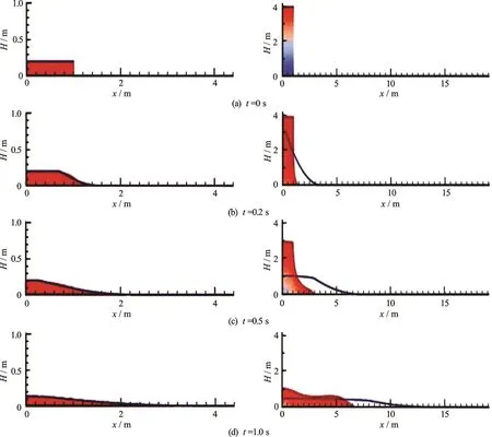
Fig.5 (Color online) Comparison of the dam-break flow simulations (left: =0.2a , right: =4.0a ) using MPM (contours) and SWEs (solid lines) models

In the MPM simulations, it is a bit hard to get the correct profile of the flood wave if we focus only on the positions of individual water particles. To deal with this limitation, we have proposed that, for MPM simulations, the flow front position is not defined only as the position of the particle at the most front, but is defined as the position of the most front particle with continuous stream of particles following it. Hence, the small number of dispersed particles at the most front are ignored in the analysis. Because of this, the flow front positions are not obtained directly from the calculation file, but are determined from the visualization of the simulation where some errors can be introduced. Moreover, in this case study, the development trend of the flow front difference, rather than the absolute thre-shold value of the difference, should be emphasised. The development trend is what we use to evaluate the agreement of the MPM simulations and the results of SWEs in the long-term prediction. For this reason,a =1 can be regarded as the critical value for the applicability of SWEs.

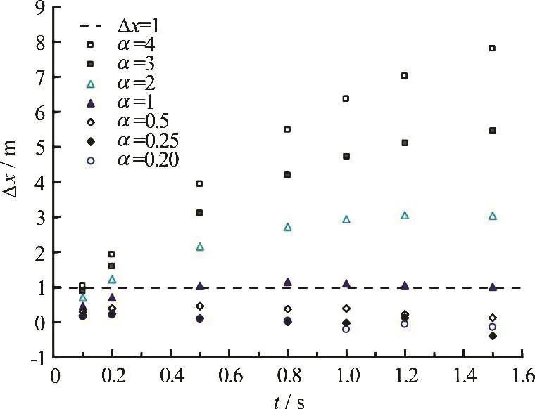
Fig.6 (Color online) Difference between flood fronts predicted by the MPM and SWEs models

In the current study, calculations are carried out on a PC using one of the four cores of an Intel®Core™i5 CPU (2.6 GHz). For a 2 s dam-break flow calculation, a SWEs simulation takes only several minutes, while a typical MPM simulation takes about 2 h depending on the computational configurations.

3. Conclusions

In this paper, the performance of the SWEs and MPM models is compared for predicting the simple dam-break flows, using the experimental data and other widely-used numerical methods (SPH, VOF) as references. The following conclusions can be drawn from this study.

(1) Compared with experimental data and other verified numerical models (SPH and VOF), the MPM simulations can give fairly good predictions of the pressure distribution and the front propagation of dambreak floods.

(2) The selection of the mesh size and number of material points per element shows insignificant effect on the dam-break flow modelling.

(3) For aspect ratio 1a£ , the SWEs can accurately capture the front movement of the dam-break flows, for 1a> , the SWEs predictions of the flood front movement are no longer reliable. It tends to overestimate the propagation speed of the dam-break flows. Hence, the critical aspect ratio for the applicability of the SWEs can be regarded to be 1.

(4) With regard to the computational cost, the SWEs solver is much more efficient than the MPM. In other words, the SWEs solver still has its advantage in predicting the propagation of dam-break flows with small aspect ratios for its efficiency. The present SPH simulations are also shown to be more efficient than the MPM simulations, although their computational costs are of the same order of magnitude.

Acknowledgements

The research is supported by the European Union Seventh Framework Program (FP7/2007-2013) under grant agreement No. PIAG-GA-2012-324522“MPM-DREDGE”. We are also grateful to a Ph. D. Placement grant made available by the British Council Newton Fund.

[1] Brackbill J. U., Kothe D. B., Ruppel H. M. FLIP: A lowdissipation, particle-in-cell method for fluid flow [J]. Computer Physics Communications, 1988, 48(1): 25-38.

[2] Sulsky D., Zhou S. J., Schreyer H. L. Application of a particle-in-cell method to solid mechanics [J]. Computer Physics Communications, 1995, 87(1-2): 236-252.

[3] Sulsky D., Chen Z., Schreyer H. L. A particle method for history-dependent materials [J]. Computer Methods in Applied Mechanics and Engineering, 1994, 118(1-2): 179-196.

[4] Bardenhagen S. G., Kober E. M. The generalized interpolation material point method [J]. Computer Modeling in Engineering and Sciences, 2004, 5(6): 477-495.

[5] Zhang H. W., Wang K. P., Chen Z. Material point method for dynamic analysis of saturated porous media under external contact/impact of solid bodies [J]. Computer Methods in Applied Mechanics and Engineering, 2009, 198(17-20): 1456-1472.

[6] Alonso E. E., Zabala F. Progressive failure of Aznalcóllar dam using the material point method [J]. Géotechnique, 2011, 61(9): 795-808.

[7] Jassim I., Stolle D., Vermeer P. Two-phase dynamic analysis by material point method [J]. International Journal for Numerical and Analytical Methods in Geomechanics, 2013, 37(15): 2502-2522.

[8] Abe K., Soga K., Bandara S. Material point method for coupled hydromechanical problems [J]. Journal of Geotechnical Engineering, 2013, 140(3): 04013033.

[9] Bandara S., Soga K. Coupling of soil deformation and pore fluid flow using material point method [J]. Computers and Geotechnics, 2015, 63: 199-214.

[10] Zhao X., Liang D. MPM Modelling of seepage flow through embankments [C]. 26th International Ocean and Polar Engineering Conference. Rhodes, Greece, 2016, 1161-1165.

[11] Ma S., Zhang X., Qiu X. M. Comparison study of MPM and SPH in modeling hypervelocity impact problems [J]. International Journal of Impact Engineering, 2009, 36(2): 272-282.

[12] Liang D. Evaluating shallow water assumptions in dambreak flows [J]. Proceedings of the Institution of Civil Engineers Water Management, 2010, 163(5): 227-237.

[13] Shao S., Lo E. Y. M. Incompressible SPH method for simulating Newtonian and non-Newtonian flows with a free surface [J]. Advances in Water Resources, 2003, 26(7): 787-800.

[14] Liang D., Falconer R. A., Lin B. Improved numerical modelling of estuarine flows [J]. Proceedings of the Insti-tution of Civil Engineers–Maritime Engineering, 2006, 159(1): 25-35.

[15] Fraccarollo L., Toro E. F. Experimental and numerical assessment of the shallow water model for two-dimensional dam-break type problems [J]. Journal of Hydraulic Research, 1995, 33(6): 843-864.

[16] Liang D., Lin B., Falconer R. A. A boundary-fitted numerical model for flood routing with shock-capturing capability [J]. Journal of Hydrology, 2007, 332(3-4): 477-486.

[17] Liang D., Lin B., Falconer R. A. Simulation of rapidly varying flow using an efficient TVD–MacCormack scheme [J]. International Journal for Numerical Methods in Fluids, 2007, 53(5): 811-826.

[18] Martin J. C., Moyce W. J. An experimtal study of the collapse of liquid columns on a rigid horizontal plane [J]. Philosophical Transactions of the Royal Society of London. Series A, 1952, 244(88): 312-324.

[19] Hirt C. W., Nichols B. D. Volume of fluid (VOF) method for the dynamics of free boundaries [J]. Journal of Computational Physics, 1981, 39(1): 201-225.

10.1016/S1001-6058(16)60749-7

February 7, 2017, Revised March 17, 2017)

*Biography:Xuanyu Zhao, Male, Ph. D. Candidate

Dongfang Liang,

E-mail: d.liang@eng.cam.ac.uk