Dynamic Responses of Atmospheric Carbon Dioxide Concentration to Global Temperature Changes between 1850 and 2010

Weile WANGand Ramakrishna NEMANI

1Department of Science and Environmental Policy,California State University at Monterey Bay,Seaside,CA 93955,USA

2Earth Science Division,NASA Ames Research Center,Moffett Field,CA 94035,USA

3NASA Advanced Supercomputing Division,NASA Ames Research Center,Moffett Field,CA 94035,USA

Dynamic Responses of Atmospheric Carbon Dioxide Concentration to Global Temperature Changes between 1850 and 2010

Weile WANG∗1,2and Ramakrishna NEMANI3

1Department of Science and Environmental Policy,California State University at Monterey Bay,Seaside,CA 93955,USA

2Earth Science Division,NASA Ames Research Center,Moffett Field,CA 94035,USA

3NASA Advanced Supercomputing Division,NASA Ames Research Center,Moffett Field,CA 94035,USA

Changes in Earth's temperature have significant impacts on the global carbon cycle that vary at different time scales,yet to quantify such impacts with a simple scheme is traditionally deemed difficult.Here,we show that,by incorporating a temperature sensitivity parameter(1.64 ppm yr-1◦C-1)into a simple linear carbon-cycle model,we can accurately characterize the dynamic responses of atmospheric carbon dioxide(CO2)concentration to anthropogenic carbon emissions and global temperature changes between 1850 and 2010(r2＞0.96 and the root-mean-square error＜1 ppm for the period from 1960 onward).Analytical analysis also indicates that the multiplication of the parameter with the response time of the atmospheric carbon reservoir(～12 year)approximates the long-term temperature sensitivity of global atmospheric CO2concentration (～15 ppm◦C-1),generally consistent with previous estimates based on reconstructed CO2and climate records over the Little Ice Age.Our results suggest that recent increases in global surface temperatures,which accelerate the release of carbon from the surface reservoirs into the atmosphere,have partially offset surface carbon uptakes enhanced by the elevated atmospheric CO2concentration and slowed the net rate of atmospheric CO2sequestration by global land and oceans by～30% since the 1960s.The linear modeling framework outlined in this paper thus provides a useful tool to diagnose the observed atmospheric CO2dynamics and monitor their future changes.

atmospheric CO2dynamics,climate-carbon interactions,climate change,carbon cycle

1.Introduction

Anthropogenic carbon dioxide(CO2)emissions from fossil-fuel usage and land-use changes have been almost exponentially increasing since the Industrial Revolution(Fig. 1).Their accumulation in the atmosphere appears to be changing Earth's climate(IPCC,2013),yet the full strength of anthropogenic CO2emissions for changing the climate has not been reached.Only 41%-45%of the CO2emitted between 1850 and 2010 remained in the atmosphere,while the rest was sequestered by lands and oceans(Jones and Cox, 2005;Canadell et al.,2007;Raupach et al.,2008;Knorr, 2009;also see Fig.1 of this study).This largely constant ratio,generally referred to as the“airborne fraction”(denoted as“α”in this paper),was conventionally used to evaluate the efficiency of global carbon sinks in assimilating the extra CO2from the atmosphere(Jones and Cox,2005;Canadell et al.,2007).However,recent studies indicate that the airborne fraction can be influenced by other factors and thus may notbe an ideal indicator for monitoring changes in the carbon sink efficiency(Knorr,2009;Gloor et al.,2010;Fr¨olicher et al.,2013).The calculation of the airborne fraction also neglects important responses of the global carbon cycle to climate changes.Global surface temperature has increased by～1◦C since the beginning of the 20th century(Hansen et al., 1999;Brohan et al.,2006).Given the tight coupling between temperature and the carbon cycle,the warming alone can release a large amount of CO2from the land and the oceans into the atmosphere,redistributing carbon among these reservoirs(Keeling et al.,1995;Joos et al.,1999,2001;Lenton, 2000;Friedlingsteinetal.,2006;BoerandArora,2009,2013; Rafelski et al.,2009;Frank et al.,2010;Willeit et al.,2014). Such climatic impacts need to be accounted for in order to diagnose and monitor changes in the global carbon cycle.

Previous studies have noticed that the effects of temperature on atmospheric CO2vary at different time scales,ranging from 1-2 ppm◦C-1at the scale of years to 10-20 ppm◦C-1over centuries or millennia(Woodwell et al.,1998). The long-term temperature sensitivity of atmospheric CO2is usually estimated by examining the correlations between ice-core CO2measurements and reconstructed paleoclimaticrecords before the industrial era,which comprise negligible anthropogenic influence(Woodwell et al.,1998;Scheffer et al.,2006;L¨uthi et al.,2008;Lemoine,2010;Frank et al.,2010).The short-term sensitivity is estimated from contemporary observations of temperature and atmospheric CO2(Keelingetal.,1995;AdamsandPiovesan,2005;Wangetal., 2013),which provide the necessary high temporal resolutions for the task.Because the contemporary atmospheric CO2records are strongly influenced by growing anthropogenic carbon emissions,the trends in the CO2and temperature time series often need to be removed before the data are used in correlation analysis(Wang et al.,2013).This“de-trending”process,however,inhibits the estimation of the long-term relationshipbetweenthetwofieldsbyconventionalcorrelationbased methodology.

©Institute of Atmospheric Physics/Chinese Academy of Sciences,and Science Press and Springer-Verlag Berlin Heidelberg 2016

Fig.1.Time series of global anthropogenic CO2emissions(red line),atmospheric CO2concentrations(green line),and the anomalous CO2fluxes induced by warming surface temperatures (gray shading)between 1850 and 2010.The top panel indicates the accumulated CO2fluxes or the total concentration changes,while the bottom panel shows them at annual steps.The thick and thin lines indicate long-term and interannual variations of the time series,respectively.The mathematical symbols are the same as in Eq.(1)and explained in the text.In both annual and accumulative cases,CO2emissions largely increase as an exponential function of time,while changes in the atmospheric CO2concentration are proportional to the corresponding emissions by a factor of about 0.41-0.45.

The timescale-dependent temperature sensitivity of atmospheric CO2concentration has also been suggested by modeling studies.By driving an earth system model of intermediate complexity with idealized periodic forcing,Willeit et al.(2014)found that the simulated temperature sensitivities of atmospheric CO2range from 1-4 ppm◦C-1at interannual and decadal scales to 5-12 ppm◦C-1at centennial scales,which are generally consistent with observation-based estimates(e.g.,Woodwell et al.,1998).However,model results are prone to uncertainties induced by different representations of carbon cycle processes and different initial state conditions in the simulations.For instance,the centennial temperature sensitivities of atmospheric CO2estimated from an ensemble of CMIP5(Coupled Model Intercomparison Project Phase 5)models show a wide range from 7 to 30 ppm◦C-1(Arora et al.,2013;Willeit et al.,2014).Observational constraints are thus required by models to derive more realistic results(Cox et al.,2013).

In this study,we explore a simple linear scheme to quantify the dynamic responses of global atmospheric CO2concentrationtoanthropogeniccarbonemissionsandglobaltemperature changes based on observational records.Although the coupled climate-carbon system is nonlinear in nature,it can be linearized around a(relatively)steady point within a neighborhood in its state space(Khalil,2001),which is evident in the fact that the atmospheric CO2concentration and the corresponding global climatology had been relatively stable for thousands of years before the industrial era(IPCC, 2013).The literature is rich with respect to the application of linear models to study the dynamics of the global carbon cycle or to diagnose its characteristics(e.g.,Oeschger and Heimann,1983;Maier-Reimer and Hasselmann,1987; Enting and Mansbridge,1987;Wigley,1991;Jarvis,2008; Boer and Arora,2009,2013;Gloor et al.,2010;Joos et al., 1996,2013).In particular,these previous studies suggest that the characteristic impulse response function(IRF)-or more generally,the Green's function-of a complex carbon-cycle model to external disturbances of carbon emissions, can be captured by a few linear modes(Maier-Reimer and Hasselmann,1987;Young,1999;Joos et al.,1996,2013). The states of atmospheric CO2calculated through convolutions of the simplified IRF and records of CO2emissions agree well with the corresponding simulations of the“parent”carbon cycle model(Wigley,1991;Li et al.,2009). However,few studies(if any)have studied the dynamic responses of atmospheric CO2to disturbances of temperature changes using linear models,which is a main interest of this paper.

This study also intends to address a couple of important issues that,to the knowledge of the authors,have not been rigorously discussed in the literature on the development of simple diagnostic models for the global carbon cycle.One such issue is the determination of key state variables to include in the models so that they will not neglect important dynamic features of the real-world system.For instance,a common approach in the literature has been to represent the net carbon flux from the atmosphere to the surface as a linear term that depends on the anomalous atmospheric CO2concentration and the residence time of such anomalies(e.g., Gloor et al.,2010;Raupach et al.,2014).Sometimes,an additional term is also included to account for the residual fluxes from processes such as reforestation(Rayner et al., 2015).However,the surface carbon storage as a state variable(or variables)has tended to be neglected in these studies.The diagnostic framework developed in Boer and Arora (2009,2013)explicitly considers the feedbacks of a warming climate on the global carbon cycle;but it also neglects the influence of the surface reservoirs on the atmosphere.Because variations of surface carbon reservoirs play a fundamental role in regulating carbon fluxes from the surface to the atmosphere,their absence in these previous models leads to significant restrictions on the simulated carbon cycle dynamics.Indeed,because of these restrictions,some previously reported results should be interpreted with caution(see below).

Another practical factor to decide upon in developing a diagnostic model is the complexity of the linear tool itself. Initial evaluation of the observational datasets used in this study indicates that they only allow the retrieval of a few independent system parameters(see below).Therefore,in the main text we only demonstrate our analytical framework by a simple two-box model that represents carbon exchanges between the atmosphere and the surface(i.e.,land and ocean) reservoirs.Although such a“toy”model may sit at the lowest rank in the hierarchy of global carbon cycle models(Enting,1987),its simplicity does not prevent it from shedding light on important and less well-known characteristics of the atmospheric CO2dynamics.The use of a simple model by no means implies a compromise in the scientific rigor of our findings,which we analytically verified with a generalized linear model comprised of an arbitrary large number of carbon reservoirs.For the sake of simplicity,these analytical proofs are not supplied with this paper,but will be published separately in the future.

Finally,throughout the analysis we also compare the resultsobtainedfromthetwo-boxmodeltothosefromthemore advanced Bern model(Siegenthaler and Joos,1992;Enting et al.,1994;IPCC,1996,2001).The Bern model couples the atmosphere with a process-based ocean biogeochemical scheme(Siegenthaler and Joos,1992;Shaffer and Sarmiento, 1995;Joos et al.,1999)and a multi-component terrestrial biosphere module(Siegenthaler and Oeschger,1987).The original Bern model does not consider the effects of changing global temperatures on terrestrial ecosystem respiration, which plays an important role in regulating the variability of the global carbon cycle at interannual to multidecadal time scales(Woodwell et al.,1998;Rafelski et al.,2009;Willeit et al.,2014).Therefore,we revised the Bern model to account for the effects of temperature on terrestrial ecosystem respiration and subsequently recalibrated the model(see Appendix for details).The global carbon cycle processes described in the Bern model help us diagnose the biogeochemical mechanisms underlying the characteristics of the atmospheric CO2dynamics identified with our simple linear model.

2.Datasets

The annual atmospheric CO2concentration data from 1850 to 1960 are based on the ice core CO2records from Law Dome,Antarctica(Etheridge et al.,1996),and those between1960and2010arecompiledfromtheNOAA(National Oceanic and Atmospheric Administration)Earth System Research Laboratory(ESRL)(Conway et al.,1994;Keeling et al.,1995).We merged the data following the approach described in Le Qu´er´e et al.(2009)and calculated the annual CO2growth rate as the first-order difference of the yearly CO2concentrations.Long-term records of anthropogenic CO2emissions from fossil fuel burning and cement production compiled by Boden et al.(2011),and those of landuse changes from Houghton(2003)were both downloaded from the Carbon Dioxide Information Analysis Center at Oak Ridge National Laboratory,TN,USA(http://cdiac.ornl.gov). Two sets of monthly surface temperature data are used,including GISTEMP(GISS Surface Temperature Analysis) from the NASA(National Aeronautics and Space Administration)Goddard Institute for Space Studies(Hansen et al.,1999)and the CRU-NCEP(Climatic Research Unit-National Centers for Environmental Prediction)climate dataset(Sitch et al.,2008;Le Qu´er´e et al.,2009),available from 1901 to the present with spatial resolutions of 0.5◦×0.5◦(CRU-NCEP)or 1◦×1◦(GISTEMP).Monthly time series of temperature are aggregated globally and over the tropics(24◦N-24◦S),and smoothed with a 12-month running window to convert the monthly data to annual values. We calculated temperature anomalies relative to their 1901 to 1920 annual mean and assumed the 20-year mean temperature to be representative of temperature climatologies between 1850 and 1900.This assumption is reasonable,as suggested by analysis of other long-term coarse-resolution temperature datasets(Jones and Moberg,2003;Brohan et al., 2006).

3.Derivation of the two-box model

Thisstudyconsidersonlythe“fast”carbonflowsbetween the atmosphere and the surface at time scales within hundreds of years(IPCC,2001).Our two-box approach treats the atmosphere as one carbon reservoir(“box”)and the world's land and oceans as the other one.Following the mathematical notation developed in Boer and Arora(2009,2013),we describe the linearized two-box carbon system as follows:

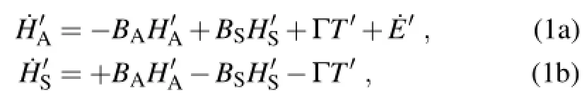
where HAand HSdenote carbon storages in the atmosphere and the surface reservoirs,with the subscripts“A”and“S”indicating the corresponding reservoirs,respectively.E is the accumulated anthropogenic CO2emissions since the industrial era.The three variables can be measured by the same unit of parts per million by volume(1 ppm=～2.13×1015grams of carbon,or 2.13 PgC).The prime symbol(e.g.,“E′”) indicates anomalies of a variable relative to its preindustrial steady-state level.The preindustrial emissions are assumed negligible so that(this assumption does not affect the results reported in this paper).The dot accentindicates the first-order derivative with regard to time,such thatrepresents the annual rate of CO2emissions(ppm yr-1). The positive parameters BAand BS(yr-1;note that“B”is the uppercase Greek letter“beta”)describe the decaying rates of corresponding carbon anomalies.Their reciprocals(i.e., τA=1/BA,τS=1/BS)are often referred to as the response time of the carbon reservoirs(IPCC,2001).T(◦C)denotes indices of global(or large-scale)surface temperatures and the parameter Γ(ppm yr-1◦C-1)indicates the rate at which carbon fluxes are released from the surface reservoirs to the atmosphere per unit change in temperature.The Γ parameter does not necessarily represent the responses of atmospheric CO2concentration to temperature changes,for the estimation of the latter must also take the dynamics of the system into account.This study assumes all three parameters(BA,BS, and Γ)to be constant,which is found to be a good approximation for the global carbon cycle over the time period under investigation(see below).

Because mass(carbon)is conserved in the two-box model,Eqs.(1a)and(1b)are not independent.Adding the two equations together,we can easily see that

which simply states that the anthropogenically emitted CO2either resides in the atmosphere or in the surface reservoirs (i.e.,the land and the oceans).Substituting this relationship into Eq.(1a)to replacewe obtain

Therefore,the dynamics of atmospheric CO2represented by the two-box model is determined by an ordinary differential equation ofunder the disturbances of anthropogenic emissionsand the changing climate(T′).

4.Model determination and evaluation

To determine the parameters of Eq.(2a)with observational records of H′A,T′and E′,we rearrange the equation, as follows,to construct a regression model:

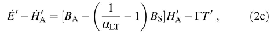
which implies that only a combination of BAand BScan be estimated from the regression analysis.Our estimate of the overallcoefficientBA-(1/αLT-1)BSis0.04±0.001(yr-1), whileαLTis separately estimated to be 0.41(Fig.1).

Additional information is required to resolve BAand BS. One source of such additional information comes from previous studies based on the measurements of carbon isotope ratios in wood and marine material(Revelle and Suess,1957), from which the response time(τA)of atmospheric CO2is inferred to be on the order of 10 years.We can also extract information from process-based model studies.BecauseτAdetermines the initial decaying rate of the IRF of a global carbon cycle model(see the proof outlined in the next section), applying this result to analyze the ensemble IRFs reported in Joos et al.(2013)suggestsτAto be～14 years.In this study, we chooseτAto be 12 years(BA≈0.083 yr-1)so that theIRF of our linear model closely matches with the Bern model during the initial decaying stage(see the next section).Subsequently,we estimateτSto be～34 years(BS≈0.029 yr-1).

The estimation of the Γ parameter in Eq.(2c)requires the choice of a large-scale temperature index that is representative of climate change and closely related with the global carbon cycle.Our previous study shows that the land surface air temperature in the tropics(24◦S-24◦N)is most strongly coupled with the interannual variations of the growth rate of atmospheric CO2by a sensitivity(Γ)of～1.64±0.28 ppm yr-1◦C-1(Wang et al.,2013).Here,we find the same temperature sensitivity parameter to be valid for Eq.(2c).Indeed, because the system is linear,variations of all the variables in Eq.(2c)over different time scales must satisfy the equation separately.Because the interannual variations(“IAV”)of the carbon emissions(˙E′and E′)and the atmospheric CO2concentration(H′A)are relatively small(Fig.1),neglecting them in Eq.(2c)leads to

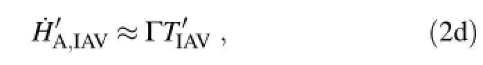
which is the same linear relationship used in Wang et al. (2013)and other previous studies(Adams and Piovesan, 2005).In addition,because the long-term trends in global temperatureand atmospheric CO2concentrations(r≈0.9)are significantly correlated,estimating Γ directly from Eq.(2c)is also subject to the influence of the collinearity between the two fields.This practical concern also makes it more reasonable to estimate Γ based on Eq.(2d)than Eq. (2c).

With the above parameters determined,we use the twobox model to simulate changes in atmospheric CO2concentration between 1850 and 2010 from historical records of temperature and carbon emissions(Fig.2).The results reproduce the evolution of the observed CO2time series to a high degree of accuracy,capturing more than 96%of the variability(i.e.,r2＞0.96)of the latter(Fig.2).The standard deviations(σ)of the differences between the simulations and the measurements since 1960 are～0.9 ppm for the atmospheric CO2concentration and～0.4 ppm yr-1for its growth rate, respectively(Fig.2).These results are highly comparable to those simulated with the revised Bern model(Fig.2)or other sophisticated climate-carbon models reported in the literature(e.g.,Joos et al.,1999;Lenton,2000;Friedlingstein et al.,2006),demonstrating that the atmospheric CO2dynamics in the past one and half centuries can be properly approximated with suitable lower-order linear models.

5.Disturbance-response functions

We first check the model's responses to an impulse disturbance of anthropogenic CO2emissions.Shown in Fig.3, the initial atmospheric CO2anomaly decays relatively fast, as 60%-70%of the emitted CO2is absorbed by the surface reservoirs within 20 years of the disturbance.However,the rate of carbon assimilation by the land and the oceans slows down significantly in the following decades and eventually becomes neutral as the system approaches a steady state,suggesting that 15%-25%of the simulated CO2anomaly will likely stay in the atmosphere for thousands of years(Fig.3). These results are consistent with the findings from fully coupled climate-carbon models(Archer et al.,2009;Cao et al., 2009;IPCC,2013;Joos et al.,2013).

The IRF of the linear models can be analytically characterized.For the model of Eq.(2a),when the system approaches a(new)steady state after the disturbance,all the time derivativeswill be zero.Assuming that temperature does not change during the process,we easily obtain the steady state ofas

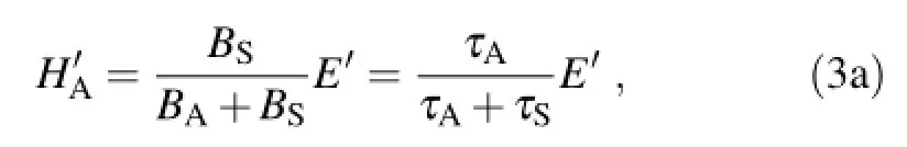
or more generally,

where the mass-conservation relationship represented by Eq. (1d)is used in the derivation.Therefore,the extra CO2added to the“fast”carbon cycle by anthropogenic emissions will be partitioned between the atmosphere and the surface corresponding to the response times(τ)of the reservoirs,respectively(Revelle and Suess,1957).BecauseτS＞τA,a majority of the emitted CO2will eventually be absorbed by the surface carbon reservoirs(Fig.3).IfτSapproaches infinity,the proportionoftheemittedCO2thatstaysintheatmospherewould decrease to zero within a few centuries,which is,however, unrealistic(IPCC,2013).This discrepancy highlights a key limitation in neglecting the influence of surface carbon storage in previous diagnostic models discussed in section 3.

The rates at which the atmospheric CO2anomaly decays are determined by the solutions(i.e.,eigenvalues)to the characteristic equation of the system.For a two-box system like Eq.(2a),the problem is particularly simple because the only non-zero eigenvalue(λ)is

and the solution of Eq.(2a)is therefore

A helpful observation of Eq.(5a)is that,when t≪1/(BA+ BS),the solution can be approximated by

Next,we consider the system's responses to disturbances induced by changes in surface temperatures.Unlike anthropogenic CO2emissions,changes in temperature do not add additional CO2to the“fast”carbon cycle,but only redistribute carbon between the atmosphere and the surface[Eqs. (1a)and(1b)],and so the system will recover to its initial steady state once the temperature anomaly is removed.However,increases in temperature are persistent under climatechange scenarios.Therefore,we examine the long-term responses of atmospheric CO2to a step change in temperature, which is easily determined from Eq.(2a)as:

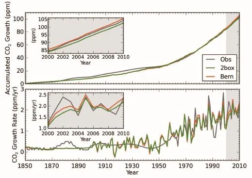
Fig.2.Simulations of the observed atmospheric CO2concentrations(top panel)and growth rates(bottom panel)from anthropogenic CO2emissions and land-surface air temperature data using the two-box model(“2box”)and the revised Bern model(“Bern”).Close-up views of the simulations between 2000 and 2010(lightly shaded)are shown in the inset figures.The atmospheric CO2concentration in 1850(i.e.,284.7 ppm)is used as the initial condition for the model integration.Long-term mean temperature before 1901 is assumed to be stable and represented by the 1901-20 mean.Other model parameters used in these simulations are explained in the main text(the two-box model)or Appendix(revised Bern model).

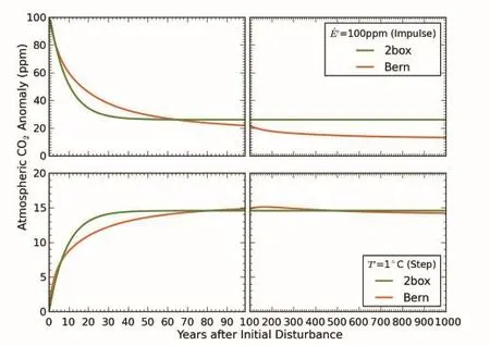
Fig.3.Disturbance-response functions of the atmospheric CO2concentration simulated by the two-box model(“2box”)and the revised Bern model(“Bern”).The top panel shows the responses of atmospheric CO2concentration to an impulse increase(of 100 ppm)in anthropogenic CO2emissions and the bottom panel shows the corresponding responses to a step increase(of 1◦C)in surface temperatures.

Because BA＞BS,for quick estimates we can also use

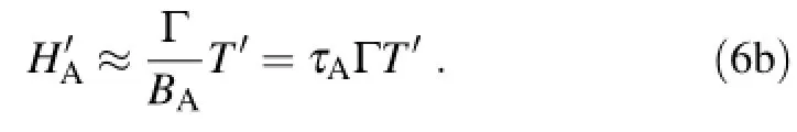
Equations(6a)or(6b)indicates that,on the first order,the long-term temperature sensitivity of atmospheric CO2concentration is largely determined by the product of the Γ parameter and the response time(τA)of the atmosphere carbon reservoir.Based on the model parameters retrieved in the preceding section,we estimate that atmospheric CO2will rise by～15 ppm for an increase of 1◦C in temperature over multidecadal to centennial time scales(Fig.3).This result generally agrees with the estimates inferred from(reconstructed) temperature and atmospheric CO2records over the Little Ice Age[～20 ppm◦C-1(Woodwell et al.,1998)],the past millennium[1.7-21.4 ppm◦C-1(Frank et al.,2010)],or estimates from coupled model experiments[5-12 ppm◦C-1(Willeit et al.,2014)].

The relationships represented by Eqs.(3b),(5b)and(6b) canbegeneralized to arbitraryhigh-orderlinearsystems.The uncertainties associated with these results-especially the long-termresponsesofatmosphericCO2-needtobeemphasized.One key source of the uncertainties is that the model's parameters are not fully determined by the observations of the global climate-carbon system.As discussed in section 4,the estimation of the model parameter BSdepends on the choice of BA,which is only loosely constrained by the prior knowledge.General analysis indicates that this situation only worsens in higher-order(N-box)systems as the number of system parameters increase by the order of N2(also see Joos et al.,1996).It is possible for us to choose another pairing of BAand BS,or a higher-order linear model,so that the derived disturbance response functions better approximate those of the Bern model(Fig.3).However,tuning the model in this fashion has only cosmetic effects on the results and does not reduce the associated uncertainties.Furthermore,in the real world,the climate system and global carbon cycle are not independent,but tightly coupled.A comprehensive assessment of the long-term fate of anthropogenic CO2emissions in the atmosphere must account for the effects of the associated changes in global temperature,which is beyond the scope of this study.

6.Biogeochemical implications

The above analysis strongly suggests that the appropriate representation of the effects of temperature on the carbon cycle in our linear model helps improve the model's accuracy in approximating the observed dynamics of the atmospheric CO2across multiple time scales.To illustrate,we further rearrange Eq.(2c)to obtain

On the left-hand side of the equation,the termis usually used to measure the net strength of annual global carbon sinks.However,because the warming temperature also releases carbon from the surface into the atmosphere(ΓT′), this extra source of CO2has to be absorbed by the global carbon sinks.By accounting for the effects of temperature changes,the termthus defines the gross global carbon sinks.

Examining Eq.(7)with the observational data shows that both the net and gross carbon sinks have been steadily increasinginresponsetotherisingatmosphericCO2concentration in the past 160 years,reaching～2.5 ppm yr-1and～4.0 ppm yr-1,respectively,in 2010(Fig.4).The gross carbon sinks have a near direct linear relationship(with a constant slope of～0.04 yr-1;r=0.98)with the atmospheric CO2concentrations throughout the entire data period.In comparison,the relationship between the apparent carbon sinks and the CO2concentrations is slightly nonlinear,with its slope decreasing from～0.03 yr-1in 1960 to～0.02 yr-1in 2010. Therefore,our linear approximation approach would not be able to achieve the same high accuracy if the effects of temperature on the carbon cycle were not correctly represented. Note that the slopes of these linear relationships are sometimes interpreted as the efficiency of surface carbon reservoirs in sequestering annual CO2emissions(Gloor et al., 2010;Raupach et al.,2014).Figure 4 shows that although the gross carbon sequestration rates BA-(1/αLT-1)BSof the surface reservoirs changed little,the net“efficiency”(the ratio betweenof the system has slowed by 28%-33%in the past five decades.This finding is essentially the same as reported in Raupach et al.(2014),but our analysis emphasizes that this declining carbon sequestration rate mainly reflects the impacts of climate changes on the global carbon cycle.Also,it must be cautioned that since the coefficient represented by BA-[(1/αLT-1)BS]is influenced by the long-term AF factor(αLT),it is not an intrinsic characteristic of the carbon cycle system.The interpretation of the coefficient as“carbon sink efficiency”is only meaningful whenαLTis constant,which is largely valid in the historical records but subject to changes in the future(IPCC,2013).

The constancy of the model parameters BA,BSand Γ needs further discussion.Previously,Boer and Arora(2009, 2013)developed a linear diagnostic framework to quantify the coefficients of CO2concentration-and temperaturerelated carbon cycle feedbacks(i.e.,BAand Γ)with the Canadian Earth System Model.Their results show long-term trends in both parameters as CO2concentration and temperature increase through the 21st century(2009,2013).To explain the discrepancies between this study and Boer and Arora(2009,2013),we notice that the term BSH′Swas neglected in the previous studies.Therefore,the“BA”parameter estimated in their studies is actually the bulk coefficient, BA-[(1/αLT-1)BS],associated with the CO2concentrationanomalyin Eq.2(c).As discussed earlier in this paper, this coefficient is sensitive to future changes in the long-term AF factor(αLT).Also,changes in atmospheric CO2concentration and global temperature are much higher under the future emission scenarios studied in Boer and Arora(2009, 2013)thanthehistoricalperiodinvestigatedinthisstudy.The changes of the parameters(BAand Γ)reported in Boer and Arora(2009,2013)may also partially reflect the fact that the global carbon cycle is gradually pushed away from its linear resilience zone in their model experiments.

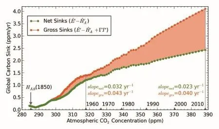
Fig.4.Global annual carbon sinks(ppm yr-1)as a function of atmospheric CO2concentration from 1850 to 2010.The green dots indicate the observed“net”carbon sinks and the red dots indicate the“gross”carbon sinks that accounted for the effects of temperature changes(Eq.7). The differences between the gross and the net carbon sinks(shaded area)indicate the extra carbon fluxes released into the atmosphere as a result of warming temperatures(Fig.1).The gray arrow(“HA,0”)indicates the estimated atmospheric CO2level(284.7 ppm)that was stable at preindustrial CO2emission rates and climate conditions.The slopes between the global annual carbon sinks and corresponding changes in atmospheric CO2concentration(relative to HA,0) were interpreted as the carbon sequestration efficiency of global land and ocean reservoirs in the literature(Gloor et al.,2010;Raupach et al.,2014).However,such an interpretation is valid only when the long-term airborne fraction(“αLT”)of anthropogenic CO2emissions is approximately constant(see discussion in the main text).

To explain the biogeochemical meaning of the Γ parameter,our previous analysis(Wang et al.,2013)suggests that it mainly reflects the temperature sensitivity of respiration of land-surfacecarbonpools(biomassandsoilcarbon).Thisexplanation is supported by the simulations of the Bern model in this study,in which terrestrial carbon sinks have much stronger responses to temperature changes than the oceanic counterpart(not shown).Furthermore,both our simulations and those from the literature(e.g.,Canadell et al.,2007;Le Qu´er´e et al.,2009)indicate that the total carbon storage in the land-surface reservoirs remains largely stable between 1850 and 2010,which is a necessary condition for Γ to be constant. For instance,because terrestrial carbon uptake accounts for 50%-60%of the global net sinks in our simulations,the accumulated terrestrial net carbon sinks are about 71-85 ppm in 2010,representing a 7%-8%increase in the total terrestrial carbon storage(～1040 ppm as of 1850).At the same time,the accumulated terrestrial carbon losses through landuse changes are about 74 ppm in 2010 based on the dataset of Houghton(2003).These results suggest that the net changes in the total terrestrial biomass and soil carbon are(relatively) small during the past 160 years,providing further justification for our linear modeling approach.

Finally,because of the buffering effect of the ocean carbonate chemistry(Revelle and Suess,1957),the responses of oceanic carbon uptake to changes in the atmospheric CO2concentration are generally estimated to be small compared with its terrestrial counterpart(e.g.,Le Qu´er´e et al.,2009). Our analysis thus suggests that the increasing atmospheric CO2concentration must have promoted carbon assimilation by the terrestrial biosphere(Ballantyne et al.,2012), most likely through the CO2fertilization effect(Long,1991; K¨orner and Arnone,1992;Oechel et al.,1994;Long et al., 2004)and the associated ecological changes(Keenan et al., 2013;Graven et al.,2013).Indeed,because the surface warming rapidly releases a proportion of the assimilated carbon back to the atmosphere(Fig.4)(Piao et al.,2008;Wang et al.,2013),the increased turnover rate may have obscured the evaluation of the magnitude of the CO2fertilization effects,which we found in calibrating the Bern model(see Appendix).In other words,the gross CO2fertilization effect of terrestrial vegetation is likely higher than previously thought(Schimel et al.,2014).

7.Conclusions

This paper develops a simple linear model to describe carbon exchanges between the atmosphere and the surface carbon reservoirs under the disturbances of anthropogenic CO2emissions and global temperature changes.We show that,with a few appropriately retrieved parameters,the model can successfully simulate the observed changes and variations of the atmospheric CO2concentration and its first-order derivative(i.e.,CO2growth rate)across interannual to multidecadal time scales.The results are highly comparable to those obtained with more sophisticated models in the literature,confirming that the simple linear model is capable of capturing the main features of atmospheric CO2dynamics in the past one and half centuries.

A distinct advantage of our linear modeling framework is that it allows us to analytically,and thus most directly,examine the dynamic characteristics of the(modeled)carbon cycle system.Our analyses indicate that many such characteristics are closely associated with the response times of the atmosphere and surface carbon reservoirs.For instance, the response time of the atmosphere determines the initial decaying rate of an impulse of CO2emitted into the atmosphere,and plays a major role in connecting the short-term and long-term temperature sensitivities of atmospheric CO2concentration.The ratio between the response times of the atmosphere and the surface reservoirs also determines the proportion of the CO2emissions that stays in the atmosphere at long-term time scales.Unfortunately,the collinearity exhibited by the observed time series of CO2emissions and atmospheric CO2concentrations has obscured the determination of the response times for individual surface reservoirs,inducing uncertainties to the estimated long-term responses of the global carbon system.

Our model results have important biogeochemical implications.They highlight that the responses of the global carbon cycle to recent anthropogenic and climatic disturbances are still within the resilience zone of the system,such that annual(gross)terrestrial and ocean carbon sinks linearly increases with the atmospheric CO2levels.On the one hand, the elevated atmospheric CO2concentration must have enhanced land carbon uptakes through the“fertilization”effects and the associated ecological changes.On the other hand,the enhanced gross carbon uptakes are partially offset by the increases in global surface temperatures,which accelerate the release of carbon from the surface reservoirs into the atmosphere.As a result,the“net”efficiency of global land and oceans in sequestering atmospheric CO2may have slowed by～30%since the 1960s,although the airborne fraction of CO2emissions remains largely constant.

Finally,and importantly,we emphasize that the linear approximationoftheglobalcarboncyclediscussedinthispaper is conditioned on the preindustrial(quasi)steady state of the system.The global climate-carbon system is clearly nonlinear beyond this scope(Archer et al.,2009),which can establishdifferentsteadystatesoverglacial/interglacialtimescales (Sigman and Boyle,2000).A major concern stemming from climate change is that,because the post-industrial anthropogenic disturbances on the global carbon cycle are so strong and rapid,they may abruptly alter the pace at which the natural climate-carbon system evolves,and drive the system into a different state at a drastically accelerated rate(IPCC,2001). Our results clearly indicate that the rising atmospheric CO2concentrations and the associated increases in global temperature have significantly intensified the global carbon cycle in the past one and half centuries.Although such intensification of the carbon system seems to be within the linear zone as of now,its resilience may be weakened,or lost,in the future.As the anthropogenic CO2emissions continue to increase and the global temperature continues to warm,scientists generally expect surface-in particular,terrestrial-carbon reservoirs to saturate and their CO2sequestration efficiency to decrease, such that the responses of the global carbon cycle to the anthropogenic disturbances will eventually deviate from their original path.With this concern in mind,the simple linear model developed in this study may serve as a useful tool to monitor the early signs of when the natural carbon system is pushed away(by anthropogenic disturbances)from its linear zone.

Acknowledgements.Wearegratefultothetwoanonymousreviewers for their constructive comments on this manuscript.This research was made possible using the NASA Earth Exchange(www. nex.nasa.gov),a“science as a service”collaborative for the geoscience community.

APPENDIX

Calibrations of the Bern Carbon Cycle Model

The Bern model is a coupled global carbon cycle box model(Siegenthaler and Joos,1992;Enting et al.,1994) that was used in previous IPCC(Intergovernmental Panel on Climate Change)Assessment Reports to study changes in atmospheric CO2concentration under different emissions scenarios(IPCC,1996,2001).It couples the High-Latitude Exchange/Interior Diffusion-Advection(HILDA)ocean biogeochemical model(Siegenthaler and Joos,1992;Shaffer and Sarmiento,1995;Joos et al.,1999)with an atmosphere layer and a multi-component terrestrial biosphere model(SiegenthalerandOeschger,1987).TheHILDAmodel describes ocean biogeochemical cycling through two wellmixed surface layers in low and high latitudes,a well-mixed deep ocean in the high latitudes,and a dissipative interior ocean in the low latitudes.Ocean tracer transport is represented by four processes:(1)eddy diffusion within the interior ocean(k,3.2×10-5m2s-1);(2)deep upwelling in the interior ocean(w,2.0×10-8m s-1),which is balanced by lateral transport between the two surface layers as well as the downwelling in the polar deep ocean;(3)lateral exchange between the interior ocean and the well-mixed polar deepocean(q,7.5×10-11s-1);and(4)verticalexchangebetween the high-latitude surface layer and the deep polar ocean(u, 1.9×10-6m s-1)(Shaffer and Sarmiento,1995).The effective exchange velocity between surface ocean layers and the atmosphere in both low and high latitudes is assumed to be the same(2.32×10-5m s-1)(Shaffer and Sarmiento,1995). Ocean carbonate chemistry(e.g.,the Revelle buffer factor)is based on the formulation given by Sarmiento et al.(1992).In addition,we implemented the influence of SST on the partial pressure of dissolved CO2in seawater with a sensitivity of～4.3%◦C-1(Gordon and Jones,1973;Takahashi et al., 1993;Joos et al.,2001).The changes in global mean SST is approximately 0.8◦C-1.0◦C from the 1850s to 2000s(Rayner et al.,2003;Brohan et al.,2006),slightly lower than that of the tropical land-based air temperature(～1.0◦C)but with a trend resembling the latter(Rayner et al.,2003;Jones and Moberg,2003;Hansen et al.,2006).For simplicity,therefore,we used the long-term trend of the tropical land air as a proxy for the corresponding trend in global SST.

The terrestrial biosphere in the Bern model is represented by four carbon compartments(ground vegetation,wood,detritus,and soil)with prescribed turnover rates and allocation ratios.The global net primary production(NPP),the influx to the biosphere,is assumed to be 60 PgC yr-1at the preindustrial level;and the effect of CO2fertilization on NPP(i.e.,the β-effect)isdescribedwithalogarithmicfunctionwithaβparameterof0.38(Entingetal.,1994).TheoriginalBernmodel does not consider the effects of changing global temperatures on terrestrial ecosystem respiration,which have been suggested to play an important role in regulating the variability of the global carbon cycle at interannual to multidecadal time scales(Rafelski et al.,2009;Wang et al.,2013).Therefore,we implemented the effects of temperature on terrestrial ecosystem respiration in the Bern model with an overall sensitivity(Q10)of～1.5(Lenton,2000;Davidson and Janssens, 2006;Wang et al.,2013).We also changed the preindustrial CO2concentration to 285 ppm in the Bern model to reflect the findings obtained from the observations(Fig.4 of the main text).

We calibrated the Bern model so that the model outputs fit the observed atmospheric CO2data most favorably.Because no major revisions were made to the ocean carbon cycle module(HILDA),we focused mainly on calibrating the biosphere module.With the original biosphere model parameters,the simulated atmospheric CO2concentrations were found to be distinctly higher than observations,reaching～411 ppm in 2010.These results are induced because rising temperatures enhance respiration in the model,reducing the net land carbon sinks to an unrealistic～0.5 ppm yr-1in 2010.To balance the temperature-enhanced respiration,we need to increase theβparameter from 0.38 to 0.64 to incorporate a higher rate of gross biosphere carbon uptake,as enhanced by CO2fertilization(Long et al.,2004)and the associated ecological changes(Keenan et al.,2013).With theβparameter set at 0.64,the simulated global terrestrial NPP increased by 14%from its preindustrial level and reached～69 PgC yr-1in 2010,which qualitatively agrees with recent estimates inferred from isotope measurements(Welp et al.,2011).As such,the recalibrated Bern model is able to simulate accurately the observed changes/variations in atmospheric CO2concentration and growth rate in the past 160 years(Fig.2 of the main text).The simulated ocean and land components of global carbon sinks are also consistent with estimates found in previous studies(e.g.,Canadell et al.,2007;Le Qu´er´e et al.,2009).

REFERENCES

Adams,J.M.,and G.Piovesan,2005:Long series relationships between global interannual CO2increment and climate:Evidence for stability and change in role of the tropical and boreal-temperate zones.Chemosphere,59,1595-1612.

Archer,D.,and Coauthors,2009:Atmospheric lifetime of fossil fuel carbon dioxide.Annual Review of Earth and Planetary Sciences,37,117-134.

Arora,V.K.,and Coauthors,2013:Carbon-concentration and carbon-climate feedbacks in CMIP5 Earth system models.J. Climate,26,5289-5314.

Ballantyne,A.P.,C.B.Alden,J.B.Miller,P.P.Tans,and J.W. C.White,2012:Increase in observed net carbon dioxide uptake by land and oceans during the past 50 years.Nature,488, 70-72.

Boden,T.A.,G.Marland,and R.J.Andres,2011:Global,regional,and national fossil-fuel CO2emissions.Carbon Dioxide Information Analysis Center,Oak Ridge National Laboratory,U.S.Department of Energy,Oak Ridge,Tenn.,U.S. A.,doi:10.3334/CDIAC/00001V2011.

Boer,G.J.,and V.K.Arora,2009:Temperature and concentration feedbacks in the carbon cycle.Geophys.Res.Lett.,36, L02704,doi:10.1029/2008GL036220.

Boer,G.J.,and V.K.Arora,2013:Feedbacks in emission-driven and concentration-driven global carbon budgets.J.Climate, 26,3326-3341.

Brohan,P.,J.J.Kennedy,I.Harris,S.F.B.Tett,and P.D.Jones, 2006:Uncertainty estimates in regional and global observed temperature changes:A new data set from 1850.J.Geophys. Res.,111,D12106,doi:10.1029/2005JD006548.

Canadell,J.G.,and Coauthors,2007:Contributions to accelerating atmospheric CO2growth from economic activity,carbon intensity,and efficiency of natural sinks.Proc.Natl.Acad. Sci.U.S.A.,104,18 866-18 870.

Cao,L.,and Coauthors,2009:The role of ocean transport in the uptake of anthropogenic CO2.Biogeosciences,6,375-390.

Chatterjee,S.,and A.S.Hadi,2006:Regression Analysis by Example.4th ed.,Wiley&Sons,408 pp.

Conway,T.J.,P.P.Tans,L.S.Waterman,K.W.Thoning,D.R. Kitzis,K.A.Masaarie,and N.Zhang,1994:Evidence for interannual variability of the carbon cycle from the National Oceanic and Atmospheric Administration/Climate Monitoring and Diagnostics Laboratory global air sampling network. J.Geophys.Res.,99,22 831-22 855.

Cox,P.M.,D.Pearson,B.B.Booth,P.Friedlingstein,C.Huntingford,C.D.Jones,and C.M.Luke,2013:Sensitivity of tropical carbon to climate change constrained by carbon dioxide variability.Nature,494,341-344.

Davidson,E.A.,and I.A.Janssens,2006:Temperature sensitivity of soil carbon decomposition and feedbacks to climate change.Nature,440,165-173.

Enting,I.G.,1987:A modelling spectrum for carbon cycle studies.Mathematics and Computers in Simulation,29,75-85.

Enting,I.G.,and J.V.Mansbridge,1987:Inversion relations for the deconvolution of CO2data from ice cores.Inverse Problems,3,L63-L69.

Enting,I.G.,T.M.L.Wigley,and M.Heimann,1994:Future emissions and concentrations of carbon dioxide:Key ocean/ atmosphere/land analyses.CSIRO Division of Atmospheric Research Technical Paper 31,CSIRO,Australia,127 pp.

Etheridge,D.M.,L.P.Steele,R.L.Langenfelds,R.J.Francey, J.-M.Barnola,and V.I.Morgan,1996:Natural and anthropogenic changes in atmospheric CO2over the last 1000 years fromairinAntarcticiceandfirn.J.Geophys.Res.,101,4115-4128.

Frank,D.C.,J.Esper,C.C.Raible,U.B¨untgen,V.Trouet,B. Stocker,and F.Joos,2010:Ensemble reconstruction constraints on the global carbon cycle sensitivity to climate.Nature,463,527-530.

Friedlingstein,P.,and Coauthors,2006:Climate-carbon cycle feedback analysis:results from the C4MIP model intercomparison.J.Climate,19,3337-3353.

Fr¨olicher,T.L.,F.Joos,C.C.Raible,and J.L.Sarmiento,2013: Atmospheric CO2response to volcanic eruptions:the role of ENSO,season,and variability.Global Biogeochemical Cycles,27,239-251.

Gloor,M.,J.L.Sarmiento,and N.Gruber,2010:What can be learned about carbon cycle climate feedbacks from the CO2 airborne fraction?Atmospheric Chemistry and Physics,10, 7739-7751.

Gordon,L.I.,and L.B.Jones,1973:The effect of temperature on carbon dioxide partial pressures in seawater.Marine Chemistry,1,317-322.

Graven,H.D.,and Coauthors,2013:Enhanced seasonal exchange of CO2by northern ecosystems since 1960.Science,341, 1085-1089,doi:10.1126/science.1239207.

Hansen,J.,R.Ruedy,J.Glascoe,and M.Sato,1999:GISS analysis of surface temperature change.J.Geophys.Res.,104,30 997-31 022.

Hansen,J.,M.Sato,R.Ruedy,K.Lo,D.W.Lea,and M.Medina-Elizade,2006:Global temperature change.Proc.Natl.Acad. Sci.U.S.A.,103,14 288-14 293.

Houghton,R.A.,2003:Revised estimates of the annual net flux of carbon to the atmosphere from changes in land use and land management 1850-2000.Tellus B,55,378-390.

IPCC,1996:Climate Change 1995:The Science of Climate Change.Contribution of Working Group I to the Second Assessment Report of the Intergovernmental Panel on Climate Change.J.T.Houghton et al.,Eds.,Cambridge University Press,Cambridge,UnitedKingdomandNewYork,NY,USA, 572 pp.

IPCC,2001:Climate Change 2001:The Scientific Basis.Contribution of Working Group I to the Third Assessment Report of the Intergovernmental Panel on Climate Change.J.T.Houghton et al.,Eds.,Cambridge University Press,Cambridge,United Kingdom and New York,NY,USA,881 pp.

IPCC,2013:Climate Change 2013:The Physical Science Basis. Contribution of Working Group I to the Fifth Assessment Report of the Intergovernmental Panel on Climate Change.T.F. Stocker et al.,Eds.,Cambridge University Press,Cambridge, United Kingdom and New York,NY,USA,1535 pp.

Jarvis,J.A.,P.C.Young,D.T.Leedal,and A.Chotai,2008:A robust sequential CO2emissions strategy based on optimal control of atmospheric CO2concentrations.Climatic Change, 86,357-373.

Jones,C.D.,and P.M.Cox,2005:On the significance of atmospheric CO2growth rate anomalies in 2002-2003.Geophys. Res.Lett.,32,L14816,doi:10.1029/2005/GL023027.

Jones,P.D.,and A.Moberg,2003:Hemispheric and large-scale surface air temperature variations:An extensive revision and an update to 2001.J.Climate,16,206-223.

Joos,F.,M.Bruno,R.Fink,U.Sigenthaler,T.F.Stocker,C.Le Qu´er´e,and J.L.Sarmiento,1996:An efficient and accurate representation of complex oceanic and biospheric models of anthropogenic carbon uptake.Tellus,48B,397-417.

Joos,F.,G.-K.Plattner,T.F.Stocker,O.Marchal,and A.Schmittner,1999:Global warming and marine carbon cycle feedbacks on future atmospheric CO2.Science,284,464-467.

Joos,F.,I.C.Prentice,S.Sitch,R.Meyer,G.Hooss,G.-K.Plattner,S.Gerber,and K.Hasselmann,2001:Global warming feedbacks on terrestrial carbon uptake under the Intergovernmental Panel on Climate Change(IPCC)emission scenarios. Global Biogeochemical Cycles,4,891-907.

Joos,F.,and Coauthors,2013:Carbon dioxide and climate impulse response functions for the computation of greenhouse gas metrics:A multi-model analysis.Atmospheric Chemistry and Physics,13,2793-2825.

Keeling,C.D.,T.P.Whorf,M.Wahlen,and J.van der Plicht, 1995:Interannual extremes in the rate of rise of atmospheric carbon dioxide since 1980.Nature,375,666-670.

Keenan,T.F.,D.Y Holligner,G.Bohrer,D.Dragoni,J.W. Munger,H.P.Schmid,and A.D.Richardson,2013:Increase in forest water-use efficiency as atmospheric carbon dioxide concentrations rise.Nature,499,324-327.

Khalil,H.K.,2001:Nonlinear Systems.3rd ed.,Princeton Hall, 750 pp.

Knorr,W.,2009:Is the airborne fraction of anthropogenic CO2emissions increasing?.Geophys.Res.Lett.,36,L21710,doi: 10.1029/2009GL040613.

K¨orner,C.,and J.A.Arnone III,1992:Responses to elevated carbon dioxide in artificial tropical ecosystems.Science,257, 1672-1675.

LeQu´er´e,C.,andCoauthors,2009:Trendsinthesourcesandsinks of carbon dioxide.Nature Geoscience,2,831-836.

Lemoine,D.M.,2010:Paleoclimatic warming increased carbon dioxide concentrations.J.Geophys.Res.,115,doi:10.1029/ 2010JD014725.

Lenton,T.M.,2000:Land and ocean carbon cycle feedback effects on global warming in a simple Earth system model.Tellus B, 52,1159-1188.

Li,S.L.,A.J.Jarvis,and D.T.Leedal,2009:Are response function representations of the global carbon cycle ever interpretable?Tellus B,61,361-371.

Long,S.P.,1991:Modification of the response of photosynthetic productivity to rising temperature by atmospheric CO2concentrations:Has its importance been underestimated?Plant, Cell&Environment,14,729-739.

Long,S.P.,E.A.Ainswroth,A.Rogers,and D.R.Ort,2004: Rising atmospheric carbon dioxide:Plants FACE the future. Annual Review of Plant Biology,55,591-628.

L¨uthi,D.,and Coauthors,2008:High-resolution carbon dioxide concentration record 650,000-800,000 years before present. Nature,453,379-382.

Maier-Reimer,E.,and K.Hasselmann,1987:Transport and storage of CO2in the ocean-an inorganic ocean-circulation car-bon cycle model.Climate Dyn.,2,63-90.

Oechel,W.C.,and Coauthors,1994:Transient nature of CO2fertilization in Arctic tundra.Nature,371,500-503.

Oeschger,H.,and M.Heimann,1983:Uncertainties of predictions of future atmospheric CO2concentrations.J.Geophys.Res., 88,1258-1262.

Piao,S.L.,and Coauthors,2008:Net carbon dioxide losses of northern ecosystems in response to autumn warming.Nature, 451,49-52.

Rafelski,L.E.,S.C.Piper,and R.F.Keeling,2009:Climate effects on atmospheric carbon dioxide over the last century.Tellus B,61,718-731.

Raupach,M.R.,J.G.Canadell,and C.Le Qu´er´e,2008:Anthropogenic and biophysical contributions to increasing atmospheric CO2growth rate and airborne fraction.Biogeosciences,5,1601-1613.

Raupach,M.R.,and Coauthors,2014:The declining uptake rate of atmospheric CO2by land and ocean sinks.Biogeosciences, 11,3453-3475.

Rayner,N.A.,D.E.Parker,E.B.Horton,C.K.Folland,L.V. Alexander,D.P.Rowell,E.C.Kent,and A.Kaplan,2003: Global analyses of sea surface temperature,sea ice,and night marine air temperature since the late nineteenth century.J. Geophys.Res.,108,doi:10.1029/2002JD002670.

Rayner,P.J.,A.Stavert,M.Scholze,A.Ahlstr¨om,C.E.Allison, and R.M.Law,2015:Recent changes in the global and regional carbon cycle:Analysis of first-order diagnostics.Biogeosciences,12,835-844.

Revelle,R.,and H.E.Suess,1957:Carbon dioxide exchange between atmosphere and ocean and the question of an increase of atmospheric CO2during the past decades.Tellus,9,18-27. Sarmiento,J.L.,J.C.Orr,and U.Siegenthaler,1992:A perturbation simulation of CO2uptake in an ocean general circulation model.J.Geophys.Res.,97,3621-3645.

Scheffer,M.,V.Brovkin,and P.M.Cox,2006:Positive feedback between global warming and atmospheric CO2concentration inferred from past climate change.Geophys.Res.Lett.,33, L10702,doi:10.1029/2005GL025044.

Schimel,D.,B.B.Stephens,and J.B.Fisher,2014:Effect of increasingCO2ontheterrestrialcarboncycle.Proc.Natl.Acad. Sci.U.S.A.,112,436-441,doi:10.1073/pnas.1407302112.

Shaffer,G.,and J.L.Sarmiento,1995:Biogeochemical cycling in the global ocean:1.A new,analytical model with continuous vertical resolution and high-latitude dynamics.J.Geophys.Res.,100,2659-2672.

Siegenthaler,U.,and H.Oeschger,1987:Biospheric CO2emissions during the past 200 years reconstructed by deconvolution of ice core data.Tellus B,39,140-154.

Siegenthaler,U.,and F.Joos,1992:Use of a simple model for studying oceanic tracer distributions and the global carbon cycle.Tellus B,44,186-207.

Sigman,D.M.,and E.A.Boyle,2000:Glacial/interglacial variations in atmospheric carbon dioxide.Nature,407,859-869.

Sitch,S.,and Coauthors,2008:Evaluation of the terrestrial carbon cycle,future plant geography and climate-carbon cycle feedbacks using five Dynamic Global Vegetation Models (DGVMs).Global Change Biology,14,2015-2039.

Takahashi,T.,J.Olafsson,J.G.Goddard,D.W.Chipman,and S.C.Sutherland,1993:Seasonal variation of CO2and nutrients in the high-latitude surface oceans:a comparative study. Global Biogeochemical Cycles,7,843-878.

Wang,W.L.,and Coauthors,2013:Variations in atmospheric CO2growth rates coupled with tropical temperature.Proc.Natl. Acad.Sci.U.S.A.,110,13 061-13 066,doi:10.1073/pnas. 1219683110.

Welp,L.R.,and Coauthors,2011:Interannual variability in the oxygen isotopes of atmospheric CO2driven by El Nino.Nature,477,579-582.

Wigley,T.M.L.,1991:A simple inverse carbon cycle model. Global Biogeochemical Cycles,5(4),373-382.

Willeit,M.,A.Ganopolski,D.Dalmonech,A.M.Foley,and G.Feulner,2014:Time-scale and state dependence of the carbon-cycle feedback to climate.Climate Dyn.,42,1699-1713.

Woodwell,G.M.,F.T.Mackenzie,R.A.Houghton,M.Apps, E.Gorham,and E.Davidson,1998:Biotic feedbacks in the warming of the Earth.Climatic Change,40,495-518.

Young,P.,1999:Data-based mechanistic modelling,generalised sensitivity and dominant mode analysis.Computer Physics Communications,117,113-129.

Wang,W.L.,and R.Nemani,2016:Dynamic responses of atmospheric carbon dioxide concentration to global temperature changes between 1850 and 2010.Adv.Atmos.Sci.,33(2),247-258,

10.1007/s00376-015-5090-y.

8 April 2015;revised 5 August 2015;accepted 17 August 2015)

∗Weile WANG

Email:weile.wang@nasa.gov