
Initial Boundary Value Problem of an Equation from Mathematical Finance∗
2016-06-09 03:34:48HuashuiZHAN
Huashui ZHAN
1 Introduction
In this paper,we consider the initial boundary value problem of the following equation:

where Ω ⊂ R2is a domain with the suitably smooth boundary ∂Ω.Equation(1.1)arises in mathematical finance(see[1]),and arises when studying nonlinear physical phenomena such as the combined effects of diffusion and convection of matter(see[2]).Antonelli,Barucci and Mancino[1]introduced a new model for the agent’s decision under risk,in which the utility function is the solution of Equation(1.1),and in particular,0≤u≤1.Under the assumption that f is a uniformly Lipschitz continuous function,Crandall,Ishii and Lions[3],Citti,Pascucci and Polidoro[4],Antonelli and Pascucci[5],step by step,proved that there is a local classical solution of Cauchy problem of Equation(1.1).
Clearly,Equation(1.1)is a strong degenerate parabolic equation since it lacks the secondorder partial derivative term∂yyu.There are some different ways to deal with the existence and uniqueness of the global weak solution of the Cauchy problem of Equation(1.1).For example,Equation(1.1)is the special case of the degenerate parabolic equations discussed in[6–7],etc.,and one can refer to[8–12]for the related results.However,Zhan[13]showed that the global weak solution of Equation(1.1)can not be classical generally.In other words,some blow-up phenomena happen in finite time.Based on these facts,we are interested in the initial boundary value problem of Equation(1.1).
It is well known that there are some rules on how to quote the initial boundary value problem of a linear degenerate parabolic equation,for which one can refer to Oleinik’s books[14–15]etc.,and we call these rules as Oleinik rules for simplicity.If Ω =(0,R)× (0,N)⊂ R2,considering the nonnegative solutions,according to Oleinik rules,and using Oleinik’s line method(see[16]),the local classical solution of Equation(1.1)has been discussed in[17].The main aim of this paper is to discuss the initial boundary value problem of Equation(1.1),provided that the spatial variables(x,y)lie in a general domain Ω ⊂ R2,and the boundary ∂Ω is suitably smooth.Certainly,the initial value condition is always required,i.e.,

To assure the well-posedness of Equation(1.1),according to Oleinik rules,we should impose

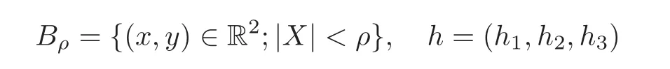
as the homogeneous boundary value condition,where

and={n1,n2,0}is the outer unit normal vector of Σ.We shall investigate the solvability of Equation(1.1)with the initial value(1.2)and the partial boundary value condition(1.3).The most important innovation of the paper lies in how to get a suitable entropy solution of(1.1)–(1.3)to arrive at its well-posedness.We shall use the general parabolic regularization method,i.e.,considering the initial boundary value problem of the following equation:

to prove the existence of the solution.In order to prove the compactness of{uε},we need some estimates on{uε}.Based on the estimates,by Kolmogoroff’s theorem,and using some ideas of[6–7]and[18],the existence of the solution is proved.
Theorem 1.1 Suppose that u0(x)∈ L∞(Ω)is suitably smooth.If fx,fy,ftare bounded functions,and fuis bounded too when u is bounded,then Equation(1.1)with the initial boundary value conditions(1.2)–(1.3)has an entropy solution.
The entropy solution in Theorem 1.1 is in the BV sense,which is defined in the following definition 2.1.Moreover,we shall use Kruzkov’s double variables method(see[19]),to discuss the stability of the solutions.Due to the complicated formula of the entropy solution defined,some special techniques are used.Beyond one’s imagination,if we consider the special domain,such as the half space Ω =R2+,or the unit disc Ω ={(x,y):x2+y2<1},then the stability of the solution may be free from the limitation of the boundary value condition.
Kobayasi K.and Ohwa H.[25]studied the well-posedness of anisotropic degenerate parabolic equations

with the inhomogeneous boundary condition on a bounded rectangle by using the kinetic formulation which was introduced in[26].Li Y.and Wang Q.[27]considered the entropy solutions of the homogeneous Dirichlet boundary value problem of(1.6)in an arbitrary bounded domain.Since the entropy solutions defined in[25,27]are only in the L∞space,the existence of the trace(defined in the traditional way,which was called the strong trace in[27])on the boundary is not guaranteed,the appropriate definition of entropy solutions are quoted,and the trace of the solution on the boundary is defined in an integral formula sense,which was called the weak trace in[27].So,not only definition 2.1 in our paper is different from the definitions of entropy solutions in[25,27],but also the trace of the solution in our paper is in the traditional way.
2 definition of the Solution
Following references[20–21],u∈BV(QT),QT=Ω×(0,T),if and only ifand

where
and K is a positive constant.This is equivalent to that the generalized derivatives of every function in BV(QT)are regular Radon measures on QT.
Let Γube the set of all jump points of u ∈ BV(QT),v be the normal of Γuat X=(x,y,t),and u+(X)and u−(X)be the approximate limits of u at X ∈ Γuwith respect to(v,Y−X)>0 and(v,Y−X)<0 respectively.For the continuous function p(x,y,t,u)and u∈BV(QT),define

which is called the composite mean value of p.For a given t,we denoteas all jump points of u(·,t),the Housdorffmeasure of,the unit normal vector of,and the asymptotic limit of u(·,t)respectively.Moreover,if f(s) ∈ C1(R)and u ∈ BV(QT),then f(u)∈BV(QT)and

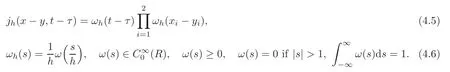
Letdτ for small η>0,whereObviously hη(s)∈ C(R)and
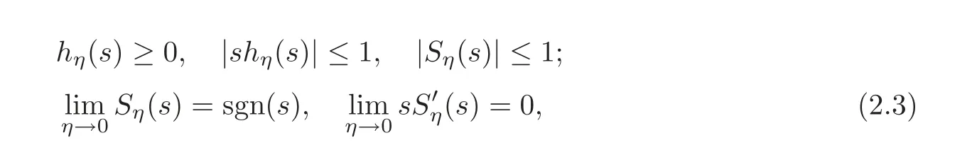
where sgn represents the sign function.
definition 2.1 A function u is said to be the entropy solution of(1.1)–(1.3),if
(1)u∈BV(QT)∩L∞(QT),and there exists a function g1∈L2(QT),such that
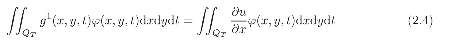
for any ϕ(x,y,t)∈ L2(QT).
(2)For any 0≤ϕ∈(QT)any k∈R,and any small η>0,u satisfies
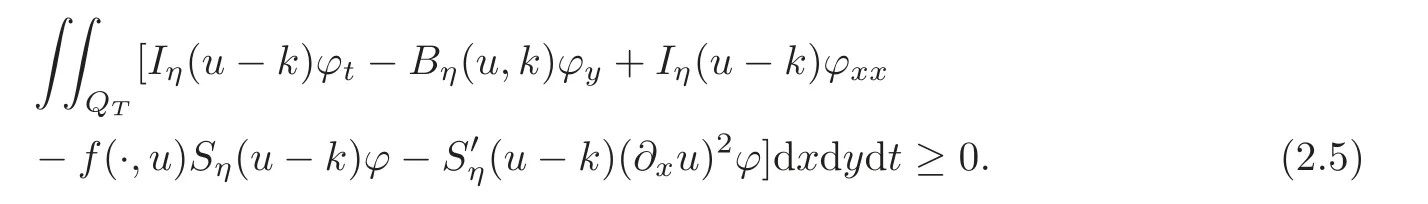
For any k∈R,η>0,here

(3)The trace on the boundary

(4)The initial value condition is true in the sense that

Clearly,by(2.5),we have

Let η→ 0 in this inequality.We have

This is just the entropy solution defined in[23–24].Thus if u is the entropy solution in definition 2.1,then u is an entropy solution defined in general cases.
3 Proof of Theorem 1.1
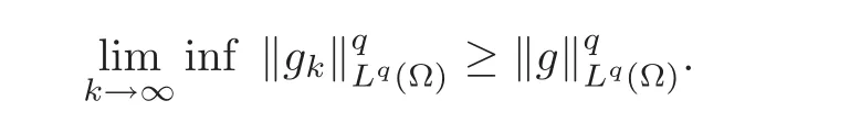
Lemma 3.1(see[28])Assume that Ω ⊂ RNis an open bounded set and let gk,f ∈ Lq(Ω),as k→∞,gk?f weakly in Lq(Ω),1≤q<∞.Then
We now consider the following regularized problem:

with the initial value(1.2)and the homogeneous boundary value condition

Under the assumptions of Theorem 1.1,it is well known that there is a classical solution uεof the initial boundary value problem of(3.1)with(1.2)and(3.2),and e.g.,one can refer to the chapter 8 of[29].
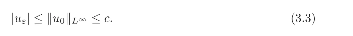
We need to make some estimates for uεof(3.1).Firstly,since u0(x)∈ L∞(Ω)is suitably smooth,by the maximum principle,we have
Secondly,let’s make the BV estimates of uε.
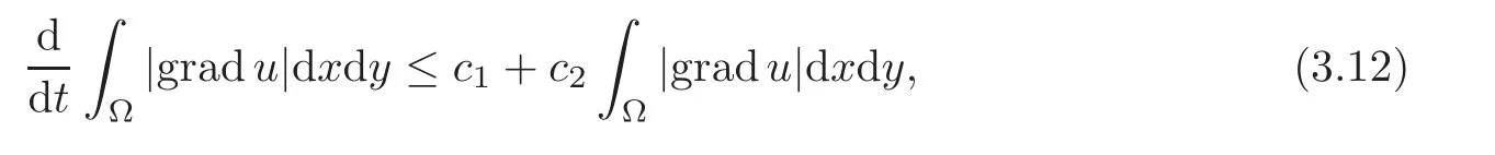
Lemma 3.2(see[18])Let uεbe the solution of(3.1)with(1.2)and(3.2).If the assumptions of Theorem 2.2 are true,then
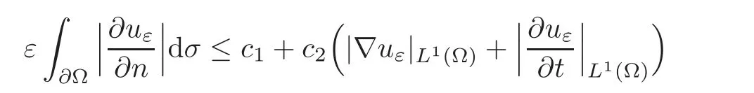
with constants ci,i=1,2 independent of ε,where={n1,n2}is the outer normal vector of Ω,and ∇uε={∂xuε,∂yuε}.
Theorem 3.1 Let uεbe the solution of(3.1)with(1.2)and(3.2).If the assumptions of Theorem 1.1 are true,then

wherec is independent of ε,and x1=x,x2=y.
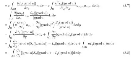
Proof In what follows,we simply denote the solution of(3.1)with(1.2)and(3.2),uε,as u,x1=x,x2=y,x3=t sometimes from the context,and the dual index of i represents the sum from 1 to 2,while the dual index of s or p represents the sum from 1 to 3.Differentiate(3.1)with respect to xs,s=1,2,3,and sum up for s after multiplying the resulting relationThen integrating over Ω yields

where ξs=uxs,and dσ is the surface integrable unit.

By the assumption that ft,fx,fyare bounded,and fuis bounded due to|u|≤c,then

From(3.5)–(3.9),we have

Observe that on Σ = ∂Ω ×[0,T),

which implies that

Let the surface integral in(3.10)be

Then,by Lemma 3.2,using(3.11),can be estimated by|gradu|L1(Ω),and one can refer to[18]for details.
Thus,by(3.10),letting η → 0,and noticing that

we have
and by the well known Gronwall lemma,we have
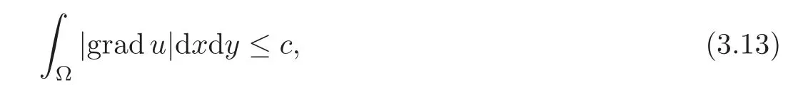
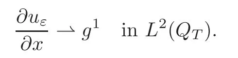
where c is a constant independent of t.By(3.13),using Equation(3.1),it is easy to show that

Now,we denote back that uεis the solution of(3.1).Thus by Kolmogoroff’s theorem,there exists a subsequence{uεn}of uεand a function u ∈ BV(QT)∩L∞(QT)such that uεnis strongly convergent to u,so uεn→ u a.e.on QT.By(3.14),there exist functions g1∈ L2(QT)and a subsequence of{ε},and we can simply denote this subsequence as ε,such that when ε→0,
We now prove that u is a generalized solution of(1.1)–(1.3).Let ϕ ∈ C20(QT), ϕ ≥ 0.Multiplying(3.1)by ϕSη(uε− k),and integrating over QT,we obtain
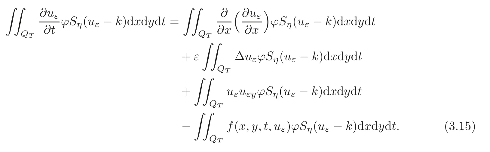
Let’s calculate every term in(3.15)by the part integral method:


From(3.15)–(3.20),we have
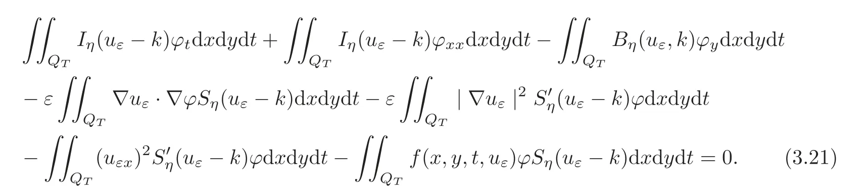
By(3.21),we have
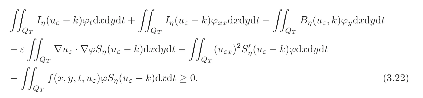
By Lemma 3.1,
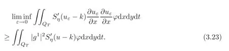
Let ε→ 0 in(3.22).By(3.23),we get(2.5).At the same time,(2.6)is naturally concealed in the limiting process.
The proof of(2.7)is similar to that in[2,6],so we omit the details here.
4 Double Variables Method
Lemma 4.1(see[6])Let u be a solution of(1.1).Then

which is true in the sense of the Hausdorffmeasure H2(Γu).
In this section,we shall prove how to use the double variables method to consider the stability of the solutions.Let u,v be two entropy solutions of(1.1)with initial values

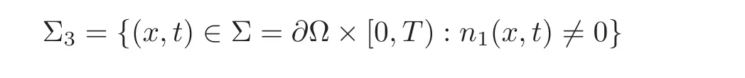
and with the homogeneous boundary value u(x,y,t)=v(x,y,t)=0 when(x,y,t)∈ Σ3.For simplicity,we denote the spatial variables(x,y)as(x1,x2)or(y1,y2)in what follows,and correspondingly,dx=dx1dx2,dy=dy1dy2.
By definition 2.1,we have

Letand
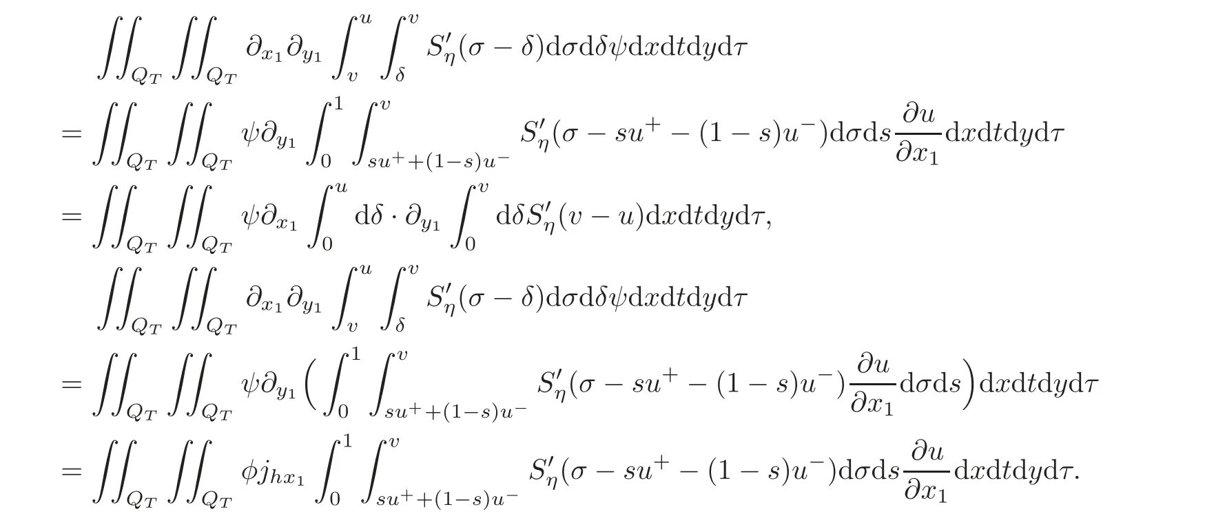
We choose k=v(y,τ),l=u(x,t), ϕ = ψ(x,t,y,τ)in(4.3)–(4.4),integrate over QT,add them together,and then we get
Clearly,
Noticing that

as η → 0,we have

and as h→0,we have
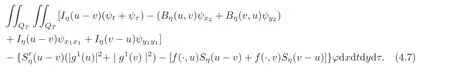
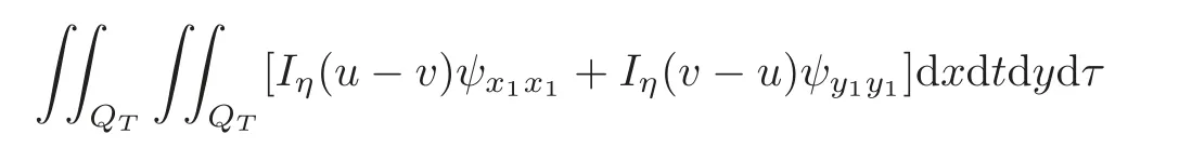
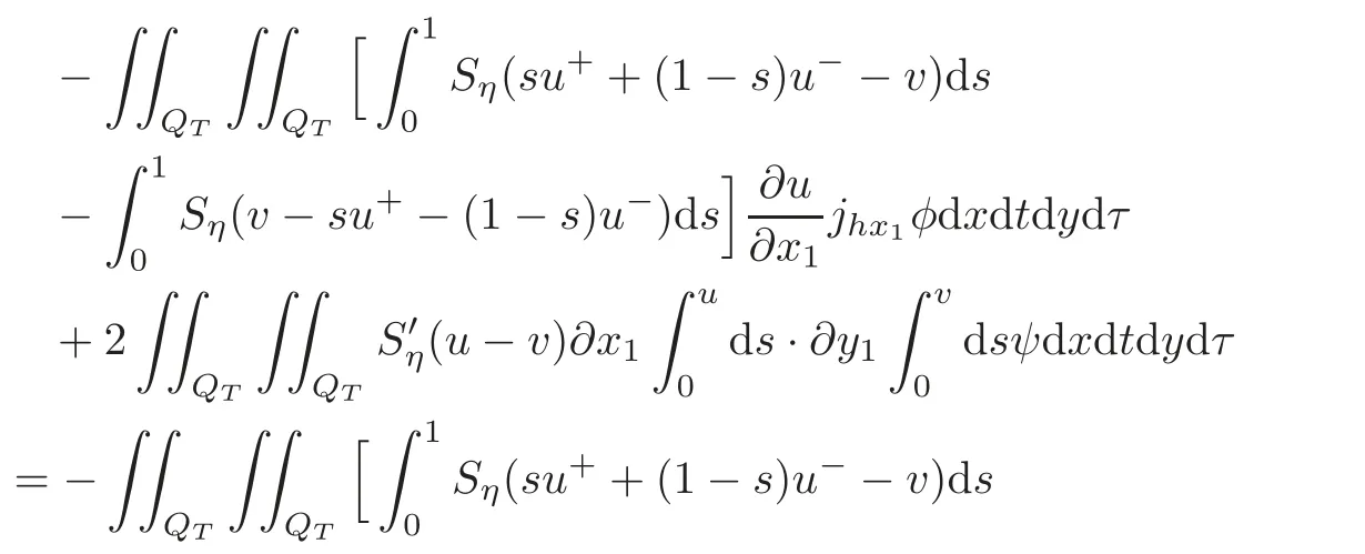
For the third term and the forth term in the bracket of(4.7),we have

Noticing that
and by the properties of the BV function(the equality(2.2)and Lemma 4.1)
We have
Noticing thatwe have

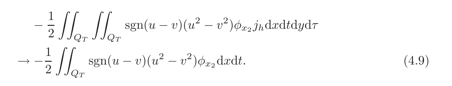
Combining(4.7)–(4.13),and letting η → 0,h → 0,we get

5 Stability of the Solutions
In the last section of this paper,we shall discuss the stability of the solutions.
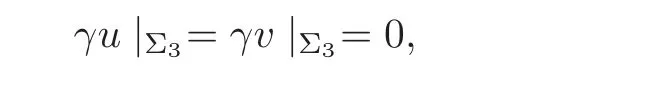
Theorem 5.1 Let 0≤u≤1,0≤v≤1 be two solutions of Equation(1.1)with the homogeneous boundary value γu|Σ3= γv|Σ3=0,and with the different initial values u0(x1,x2),v0(x1,x2) ∈ L∞(Ω)respectively.Suppose that|fu(·,u)|≤ c,and that the distance function d(x)=dist(x,∂Ω)satisfies

so then for any t∈(0,T),
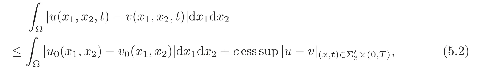
where
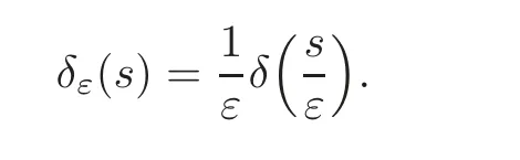
Proof Let δεbe the mollifier as usual.In detail,for the known function
where
and for any given ε>0, δε(s)is defined as
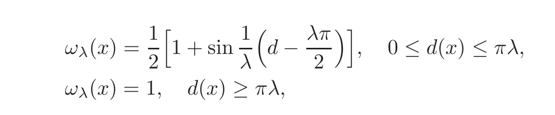
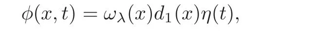
Now,we can choose φ in(4.14)by

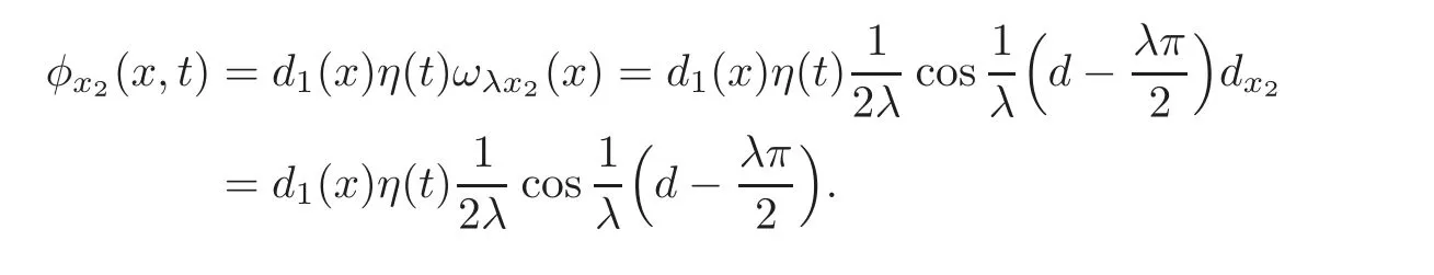
where η(t) ∈(Ω)is defined as follows.For any given small enough 0< λ,0≤ ωλ≤ 1,ω|∂Ω=0 and
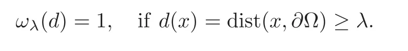
When 0≤d(x)≤λ,

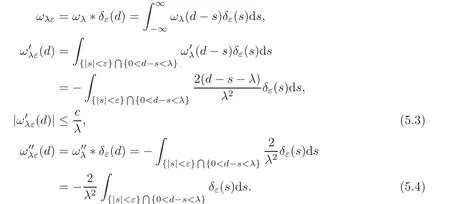
and when d<0,we let ωλ(d)=0.Then
Now,
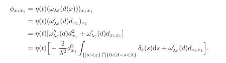
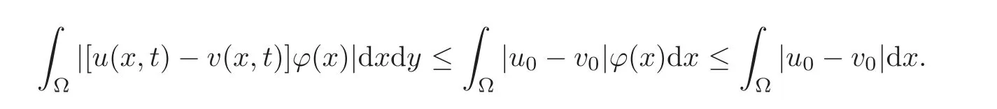
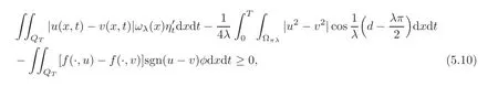
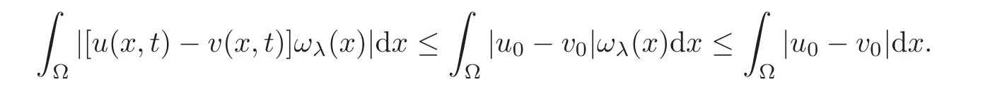
Using the condition(5.1),and|dx1x1|≤ c,and with the fact that|dxi|≤ |∇d|=1,i=1,2,0≤fu(·,u)≤ c,0 ≤ u,v ≤ 1,and from(4.14),we have

Here Ωλ={x:d(x)=dist(x,∂Ω)< λ}.By(5.3),


As λ → 0,according to the definition of the trace,by γu|Σ3= γv|Σ3=0,we have

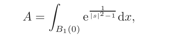
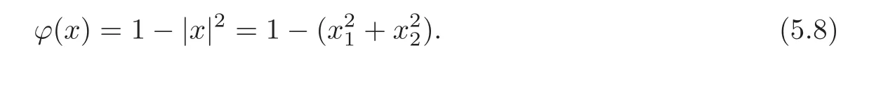
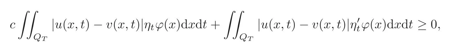
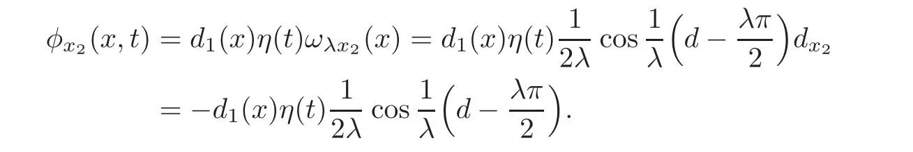
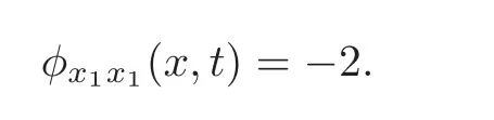
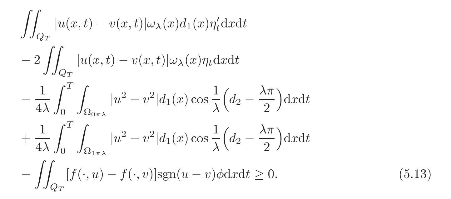
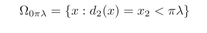
Let 0 Here α?(t)is the kernel of the mollifier with α?(t)=0 for t/∈(−?,?).Let?→0.Then By the Gronwall lemma,the desired result follows by letting s→0,i.e., So we have the conclusion. Theorem 5.2 Let u,v be two solutions of Equation(1.1)with the different initial values u0(x1,x2),v0(x1,x2)∈ L∞(Ω)respectively.0≤ u≤ 1,0≤ v≤ 1.Suppose that the domain Ω is just the unit discand suppose|fu(·,u)|≤ c.Then where Proof We can choose φ = ϕ(x)η(t)in(4.14),where η(t) ∈(0,T).Then we have Due to that 0≤u≤1,0≤v≤1,|x2|≤1, We have and as the proof of Theorem 5.1,we have Theorem 5.3 It is supposed that the domaintwo solutions of Equation(1.1)with the different initial values u0(x1,x2),v0(x1,x2)∈ L∞(Ω)∩L1(Ω)respectively.If|fu(·,u)|≤ c,then where and d(x)=dist(x,∂Ω)=x2. Remark 5.1 The condition of the initial values u0(x1,x2),v0(x1,x2)∈ L∞(Ω)∩L1(Ω)in the theorem is stronger than the solutions obtained in Theorem 1.1.At the same time,due to Ω=R2+={(x1,x2):x2>0},it implies that is an empty set.It means that the solution of the equation is free from the limitation of the boundary value in this case. Proof We can choose φ in(4.14)by whereand then From(4.14),we have whereand by(5.10),we have As the proof of Theorem 5.1,we have The proof of Theorem 5.3 is complete. At the end of this paper,let us consider a special domain Thenand let For small enough λ,we set Theorem 5.4 It is supposed that the domain Ω = ΩR.Let u,v be two solutions of Equation(1.1)with the homogeneous boundary value and with the different initial values u0(x1,x2),v0(x1,x2)∈ L∞(Ω)∈ L∞(Ω)respectively.Then Proof Through a limit process,we can choose φ in(4.14)by where When 0 When Certainly,when πλ ≤ x2≤ 1− πλ, At the same time,it is clear that From(4.14),we have Here implies implies Due to we have Letλ→0 in(5.15).As the proof of Theorem 5.1,we have the conclusion. AcknowledgementThe author expresses his sincere thanks to the reviewers for their kindly amendments to the paper. [1]Antonelli,F.,Barucci,E.and Mancino,M.E.,A comparison result for FBSDE with applications to decisions theory,Math.Meth.Oper.Res.,54,2001,407–423. [2]Escobedo,M.,Vazquez,J.L.and Zuazua,E.Entropy solutions for diffusion-convection equations with partial diffusivity,Trans.Amer.Math.Soc.,343,1994,829–842. [3]Crandall,M.G.,Ishii,H.and Lions,P.L.,User’s guide to viscosity solutions of second partial differential equations,Bull.Amer.Math.Soc.(N.S.),27,1992,1–67. [4]Antonelli,F.and Pascucci,A.,On the viscosity solutions of a stochastic differential utility problem,J.Diff.Equ.,186,2002,69–87. [5]Citti,G.,Pascucci,A.and Polidoro,S.,Regularity properties of viscosity solutions of a non-Hormander degenerate equation,J.Math.Pures Appl.,80(9),2001,901–918. [6]Zhan,H.S.,The study of the Cauchy problem of a second order quasilinear degenerate parabolic equation and the parallelism of a Riemannian manifold,Doctor Thesis,Xiamen University,2004. [7]Zhan,H.S.and Zhao,J.N.,The stability of solutions for second quasilinear degenerate parabolic equation,Acta Math.Sinica,Chinese Ser.,50,2007,615–628. [8]Chen,G.Q.and Perthame,B.,Well-posedness for non-isotropic degenerate parabolic-hyperbolic equations,Ann.I.H.Poincare-AN,20,2003,645–668. [9]Chen,G.Q.and Dibendetto,E.,Stability of entropy solutions to Cauchy problem for a class of nonlinear hyperbolic-parabolic equations,SIAM J.Math.Anal.,33,2001,751–762. [10]Karlsen,K.H.and Risebro,N.H.,On the uniqueness of entropy solutions of nonlinear degenerate parabolic equations with rough coefficient,Discrete Contain.Dye.Sys.,9,2003,1081–1104. [11]Bendahamane,M.and Karlsen,K.H.,Reharmonized entropy solutions for quasilinear anisotropic degenerate parabolic equations,SIAM J.Math.Anal.,36,2004,405–422. [12]Carrillo,J.,Entropy solutions for nonlinear degenerate problems,Arch.Rational Mech.Anal.,147,1999,269–361. [13]Zhan,H.S.,The solution of the Cauchy problem for a quasilinear degenerate parabolic equation(in Chinese),Chin.Ann.Math.Ser.A,33(4),2012,449–460. [14]Oleink,O.A.,A problem of Fichera,Dokl.Akad.Nauk SSSR,154,1964,1297–1300.Soviet Math.Dokl.,5,1964,1129–1133. [15]Oleink,O.A.,Linear equations of second order with nonnegative characteristic form,Math.Sb.,69,1966,111–140;English transl.:Amer.Math.Soc.Tranl.,65,1967,167–199. [16]Oleink,O.A.and Samokhin,V.N.,Mathematical Models in Boundary Layer Theorem,Chapman and Hall/CRC,Boca Raton,London,New York,Washington,1999. [17]Zhan,H.S.,On a quasilinear degenerate parabolic equation(in Chinese),Chin.Ann.Math.Ser.A,27(6),2006,731–740. [18]Wu,Z.and Zhao,J.,The first boundary value problem for quasilinear degenerate parabolic equations of second order in several variables,Chin.Ann.Math.Ser.B,4,1983,319–358. [19]Krukov,S.N.,First order quasilinear equations in several independent variables,Math.USSR-Sb.,10,1970,217–243. [20]Vol’pert,A.I.and Hudjaev,S.I.,On the problem for quasilinear degenerate parabolic equations of second order(in Russian),Mat.Sb.,3,1967,374–396. [21]Wu,Z.,Zhao,J.,Yin,J.and Li,H.,Nonlinear Diffusion Equations,World Scientific Publishing,Singapore,2001. [22]Zhan,H.S.,Harnack estimates for weak solutions to a singular parabolic equation,Chin.Ann.Math.Ser.B,32(3),2011,397–416. [23]Volpert,A.I.and Hudjave,S.I.,Analysis of Class of Discontinuous Functions and the Equations of Mathematical Physics,Izda.Nauka Moskwa,Martinus Nijhoff Publishers,Moscow,1975(in Russian). [24]Volpert,A.I.,BV space and quasilinear equations,Mat.Sb.,73,1967,255–302. [25]Kobayasi,K.and Ohwa,H.,Homogeneous Dirichlet problems for quasilinear anisotropic degenerate parabolic-hyperbolic equations,J.Diff.Equ.,252,2012,4719–4741. [26]Lions,P.L.,Perthame,B.and Tadmor,E.,A kinetic formulation of multidimensional conservation laws and related equations,J.Amer.Math.Soc.,7,1994,169–191. [27]Li,Y.and Wang,Q.,Uniqueness and existence for anisotropic degenerate parabolic equations with boundary conditions on a bounded rectangle,J.Diff.Equ.,252,2012,137–167. [28]Evans,L.C.,Weak convergence methods for nonlinear partial differential equations,Conference Board of the Mathematical Sciences,Regional Conferences Series in Mathematics,74,1998. [29]Gu,L.K.,Second Order Parabolic Partial differential Equations,The Publishing Company of Xiamen University,Xiamen,2002.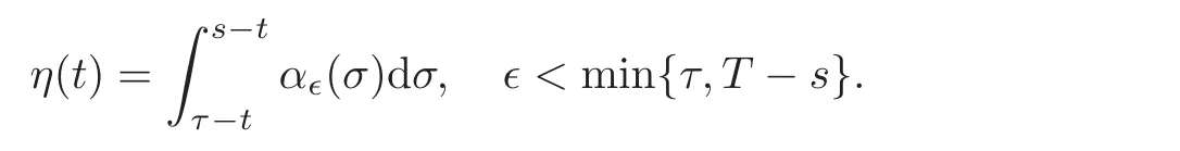


 Chinese Annals of Mathematics,Series B2016年3期