Comparison of dimension reduction-based logistic regression models for case-control genome-wide association study:principal components analysisvs.partial least squares

Honggang Yi,Hongmei Wo,Yang Zhao,Ruyang Zhang,Junchen Dai,Guangfu Jin,3, Hongxia Ma,3,Tangchun Wu,Zhibin Hu,3,5,Dongxin Lin,Hongbing Shen,3,5,Feng Chen,✉

1Department of Epidemiology and Biostatistics,School of Public Health;2Department of Public Service Management,School of KangDa;3Section of Clinical Epidemiology,Jiangsu Key Laboratory of Cancer Biomarkers,Prevention and Treatment, Cancer Center;

4Institute of Occupational Medicine and Ministry of Education,Key Laboratory for Environment and Health,School of Public Health,Tongji Medical College,Huazhong University of Science and Technology,Wuhan 430030,China;5State Key Laboratory of Reproductive Medicine,Nanjing Medical University,Nanjing,Jiangsu 211166,China;

6State Key Laboratory of Molecular Oncology and Department of Etiology and Carcinogenesis,Cancer Institute and Hospital, Chinese Academy of Medical Sciences and Peking Union Medical College,Beijing 100021,China.

Comparison of dimension reduction-based logistic regression models for case-control genome-wide association study:principal components analysisvs.partial least squares

Honggang Yi1,△,Hongmei Wo2,△,Yang Zhao1,Ruyang Zhang1,Junchen Dai1,Guangfu Jin1,3, Hongxia Ma1,3,Tangchun Wu4,Zhibin Hu1,3,5,Dongxin Lin6,Hongbing Shen1,3,5,Feng Chen1,✉

1Department of Epidemiology and Biostatistics,School of Public Health;2Department of Public Service Management,School of KangDa;3Section of Clinical Epidemiology,Jiangsu Key Laboratory of Cancer Biomarkers,Prevention and Treatment, Cancer Center;

4Institute of Occupational Medicine and Ministry of Education,Key Laboratory for Environment and Health,School of Public Health,Tongji Medical College,Huazhong University of Science and Technology,Wuhan 430030,China;5State Key Laboratory of Reproductive Medicine,Nanjing Medical University,Nanjing,Jiangsu 211166,China;

6State Key Laboratory of Molecular Oncology and Department of Etiology and Carcinogenesis,Cancer Institute and Hospital, Chinese Academy of Medical Sciences and Peking Union Medical College,Beijing 100021,China.

With recent advances in biotechnology,genome-wide association study(GWAS)has been widely used to identify genetic variants that underlie human complex diseases and traits.In case-control GWAS,typical statistical strategy is traditional logistical regression(LR)based on single-locus analysis.However,such a single-locus analysis leads to the well-known multiplicity problem,with a risk of inflating type I error and reducing power.Dimension reduction-based techniques,such as principal component-based logisticregression(PC-LR),partial least squares-based logistic regression (PLS-LR),have recently gained much attention in the analysis of high dimensional genomic data.However,the performance of these methods is still not clear,especially in GWAS.We conducted simulations and real data application to compare the type I error and power of PC-LR,PLS-LR and LR applicable to GWAS within a defined single nucleotide polymorphism(SNP)setregion.WefoundthatPC-LRandPLScanreasonablycontroltypeIerrorundernullhypothesis. Oncontrast,LR,whichiscorrectedbyBonferronimethod,wasmoreconservedinallsimulationsettings.Inparticular,we found that PC-LR and PLS-LR had comparable power and they both outperformed LR,especially when the causal SNP was in high linkage disequilibrium with genotyped ones and with a small effective size in simulation.Based on SNP set analysis,we applied all three methods to analyze non-small cell lung cancer GWAS data.

principalcomponentsanalysis,partialleastsquares-basedlogisticregression,genome-wideassociationstudy, type I error,power

Introduction

With the rapid development of high-throughput genotyping technologies in recent years,genome-wide association studies(GWAS)has emerged as popular tools for identifying genetic variants involved in complex diseases and traits[1].GWAS have identified hundreds of associations of common susceptibility loci with more than 100 complex diseases or phenotypes, including cardiovascular disease,cancer,Parkinson’s disease and type 2 diabetes[2-7].

Although our understanding of genetic basis of these complex diseases and trait has been improved,there are still many analytic challenges in GWAS[8-9].Published case-control GWAS typically used a single-locus logistic regression(LR),in which each variant is tested individually for association with a specific phenotype in the whole genome.However,such a SNP-by-SNP analysis leadstothewell-knownmultiplicityproblem,witharisk of inflating type I error and reducing power[10].One way thatwaswidelyusedtodealwiththischallengeistoperform correction,such as Bonferroni correction method, which corrects the significance level of each testing and controls the family-wide type I error.However,since many single nucleotide polymorphisms(SNPs)are in linkage disequilibrium(LD)with each other,this approach is highly conservative as we showed in our previous work[11].

Another common strategy is to utilize dimension reduction techniques,so as to improve power by using information"borrowed"from correlated SNPs,and reducing the unnecessary degree of freedom. Dimension reduction techniques,such as principal components analysis(PCA)or partial least squares (PLS),have recently gained much attention in the analysis of high-dimensional genomic data.For a binary dependent variable,Gauderman et al.introduced a PC-based logistic regression(PC-LR)to assess whether a gene region,represented by multiple SNPs,is associated with disease[12].It establishes a relationship between the binary response variable and the selected PCs of the explanatory variables.However,one important limitation of PC-LR that commonly arises is that the coefficients that make up each eigenvector lack interpretation in detail.

The PLS method is another powerful approach for the analysis of high-dimensional data.PLS regression was introduced by Wold et al.and later developed by many authors in recent years[13-14].Marx proposed PLS generalized linear regression(PLS-GLM)and particular case of PLS logistic regression(PLS-LR) for the binary output variable as an extension of PLS regression[15-16].In contrast to PC-LR which extracts orthogonal PCs solely from explanatory variables, PLS-LR creates orthogonal components by using the existing correlations between explanatory and corresponding response variable while also keeping most of the variance of explanatory.Because it allows to retain in model all variables with a stronger correlation to the response variable,it is also referred to as a kind of supervised method.PLS-GLM including PLS logistic regression has been used in the field of gene expression microarray data and classification problems in the last several years[17-19].

PC-LR and PLS-LR all have been widely used in genetic studies.An outstanding question,however,is the relative performance among these methods. Because of different algorithms and strategies,the performance and effectiveness under different situations ofthesemethodsmaybedifferent.Chunetal.compared the performance of PLS linear regression and PC linear regression[20].By now,limited comparisons have been conducted to evaluate and compare the performance of these methods,especially in SNP sets based GWAS.

In this article,we compared PC-LR and PLS-LR for SNP sets based association testing in GWAS.We also included the standard LR for comparison.We first reviewed these two methods.Then,we used the HapMap project to simulate a set of population data. Based on simulations,we assessed their performance under various scenarios,considering significant level, sample size,relative risk(RR)of disease susceptible allele and disease loci.At last,we compared these methods with a real GWAS data.This comparison allows us to explore the limitation and the power of these methods for association testing for GWAS.

Materials and methods

PC-based logistic regression(PC-LR)

Suppose that a SNP set includes p SNPs from n individuals within a gene region,where gi=(gi1,gi2,...,gik)Tdenote genotype scores of the ith individual,each code as 0,1 or 2 for observed number of minor alleles in additive mode.In our study,all genotypes were assumed to be standardized with a mean of 0 and a standard deviation of 1.Case-control status for the subjects is denoted by D(1=affected,0=unaffected).

The basic idea of PCA is to discover linear projections of the correlated SNPs with maximum variance, and use principal components(PCs)that are orthogonal and uncorrelated to each other to represent genetic variation in a gene region.

Let Vp×pdenote the variance-covariance matrix of the standardized SNPs set,and Ep×p=(e1,e2,...,ep) denote p×p-dimension eigenvectors of Vp×p.The p

eigenvalues are denoted by λ=(λ1,λ2,...,λp).For the ith individual,the principal components are:

such that the h-th eigenvalue(λh)corresponds to the h-th eigenvector(eh),and the p eigenvector elements for each eigenvalue represent the coefficients of p SNPs for each linear combination.Eigenvectors are determined to maximize the variance of PChwith the constrain that eTheh=1 and eTheh′=0,for h≠h′.The later constrain means that the covariance between PChand PCh’is equal to 0,for h≠h′.

The first PC,which is independent with the other PCs,represents the linear combination of SNPs that explains the largest fraction of the genetic variability in the gene region.Similarly,PC2explains the second largest amount of SNP variation,and so forth (λ1＞λ2＞...＞λp).

The proportion of the overall variation in each PC can be explained by:

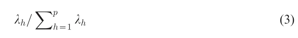
As SNPs in the set have substantial correlation among them,the first few PCs will account for most of the variation in the SNPs set.Thus,only a subset of PCs(PC1,PC2,...,PCk,k＜p)in which cumulative contribution is greater than a threshold need to be tested for association in the multiple logistic regression model:

A k-d.f.likelihood ratio test of mode(4)versus logitP(D=1)=β0provides an omnibus test of whether the SNPs set,as defined by the subset k of PCs,explains a significant proportion of the genetic variation in trait D.The value of k can be chosen such that the cumulative contributing proportion of the total variability explained by the first k PCs exceeds some threshold.In our study,different thresholds,such as 80%,60%and 40%,were performed to denote the PC-LR with the k PCs explaining the cumulative contributing proportion of the total variation,respectively.

PLS logistic regression(PLS-LR)

In the PLS-LR model,a set of latent uncorrelated variables(PLS components)were defined by linear spans of the original predictors,and then were performed as covariates of the logistic regression model. These linear spans are taken into account the relationship between the original explanatory variables and the response,and are usually obtained by nonlinear iterative partial least squares(NIPALS)algorithm[15].

PLS-LR model of D on gi=(gi1,gi2,...,gik)with m PLS components can be written as

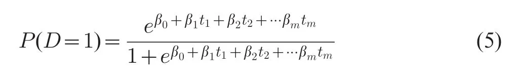
In model(5),thare the orthogonal PLS components which can be expressed by original variables(gi),and βhare partial coefficients of the m PLS components.

PLS-LR can be described by a four-step algorithm:

(1) Compute a set of PLS components;

(2) Logistic regression of the response variable on the m retained PLS components;

(3) Formulation of the PLS-LR in terms of the original explanatory variables;

(4) Bootstrap validation of coefficients in the final model of PLS-LR.

The algorithm for computing a set of PLS components follows the next steps:

(1)Computation of the first PLS component t1.To obtain the first PLS component,we will compute the partial regression coefficient a1jof gjin the logistic regression of D on gjfor each variable gj, j=1,2,...,p.Then,the column vector a1made by a1j’s are normalized by w1=a1/a1‖ ‖,and we will define the first PLS component as t1=gw1=gw*1.

(2)Computation of the second PLS component t2.To obtain the second PLS component,in a similar way, we will compute the partial regression coefficient a2jof gjin the logistic regression of D on t1and gjfor each variable gj,j=1,2,...,p.The normalized w2is estimated by a2with w2=a2/a2‖ ‖.Then,we will compute the residual matrix E1in the linear regression of gjon t1:gj=p1jt1+e1j,in which p1jis the partial coefficient of the t1,and e1jare the residuals in the model.e11,e12,...,e1jare the elements in the each column of residual matrix E1, j=1,2,...,p.The second component with t2=E1w2is computed,and expressed in terms of g:t2=gw*2, in which w*2=(I-w1p1)w2.

(3)Computation of the hthPLS component th.Given the PLS components t1,t2,...,th-1have been yielded in the previous steps,the component this obtained by iterating the search for the second component, and can be expressed by th=gw*h,where w*h=(I-Σh-1i=1w*ipi)wh.

In our study,the computation of PLS components is simplified by setting those non-significant partial regression coefficients ahjto 0.Thus,only variables that are significantly associated with D will then contribute to the computation of PLS components.The number m of PLS components to be retained are chosen by observing that the component tm+1is not significant due to none of the coefficients am+1,jis significantly different from 0.

If m PLS components are selected and expressed by original variables gj,the statistical significance of each variable gjin model(5)is done under a nonparametric framework by using a‘‘balanced bootstrap’’resampling method[16].A large,pre-specified number of subjects as the original sample were generated via resampling with replacement.All bootstrap samples together provided empirical estimation for the coefficients and their confidence intervals(CI).If the 100(1-α)%CI of each SNP’s standardized regression coefficient well below or above 0,it can be considered statistically significant.

Data simulation

Simulation studies were conducted to compare the performanceofPC-LRandPLS-LR.Theirperformances were also compared with a single-locus based LR.

Phased haplotype data sets(CHB+JPT,Han Chinese in Beijing,China and Japanese in Tokyo,Japan)were downloaded from the HapMap web site(http:// snp.cshl.org,Phase III,release 2,on NCBI B36 assembly).We selected CLPTM1-like(CLPTM1L)gene region to generate simulating genotype data.CLPTM1L,encoding cleft lip and palate transmembrane protein 1-like protein,is a 27.35 kb-long-gene located at 5p13.33.The region including±20 kb of the CLPTM1L gene is located at Chr5:1,351,007..1,418,002,including 29 SNPs.In our simulations,4 of 29 SNPs with minor allele frequency(MAF)less than 0.01 were deleted and the left 25 SNPs were used.

Based on the HapMap phased haplotype data from the CHB+JPT populations using HAPGEN2[21],100,000 cases and 100,000 controls were generated and combined to form a hypothetical population under the null hypothesis(H0)and alternative hypothesis(H1).From the population,case and control samples were randomly selected with different sample sizes N(N/2 cases and N/2 controls, N=4,000,8,000,...,20,000).Under H0,the relative risk per allele was set as 1.0 to assess type I error.Under H1, we set the different levels of relative risks(1.2,1.4,1.6 and 1.8 per allele)to assess the power.The SNPs in this region were coded according to the additive genetic model.

To investigate the performance of the three methods on different causal SNPs with different MAF and different LD patterns,each of the 25 SNPs was defined as the causal variant.To ensure that the simulations were more realistic,although all 25 HapMap SNPs were generated,only 10 of them,which were directly genotyped by Affi6.0 chip,were tested by the three methods.

From the 10 SNPs,we sampled the simulation data and performed PC-LR,PLS-LR using the R(version 2.15)packages plsRglm(http://cran.r-project. org/web/packages/plsRglm/index.html),and R functions of prcomp and glm.Under H0,we repeated 5,000 simulations at the significant level of 0.05. Under H1,for each model with a given relative risk, we repeated 1,000 simulations at four significant levels (0.05,0.01,1E-5,and 1E-7).To control the overall type I error of the single-locus LR testing in our simulation,Bonferroni correction was performed to set the significance level of the test at each locus to α/the number of SNP in the SNP set.Measurements included empirical type I error rate and test power.

Application

To demonstrate the applicability and power of PC-LR and PLS-LR on real data,we applied these two methods to real GWAS data and contrast results with those found under single-locus logistic regression analysis.

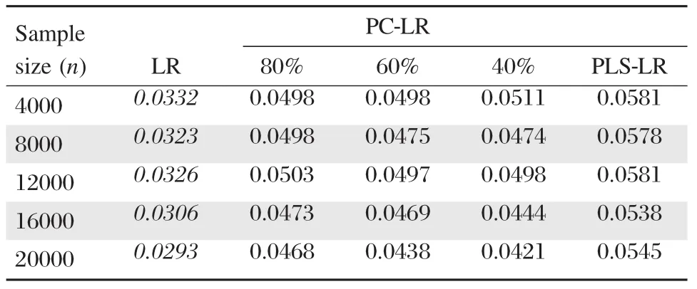
Table 1Empirical type I error rates of principal component-based logistic regression(PC-LR),PLS logistic regression(PLS-LR)and single-locus logistic regression(LR)

We mainly focused on two gene regions extracted form a non-small cell lung cancer GWAS dataset[6]. Details of participant recruitment for the study have been described previously[6].This dataset includes 5,408 subjects(2,331 individuals with lung cancer and 3,077 controls).DNA was extracted from whole blood and genotype by the Affymetrix 6.0 Quad chip. A total of 570,373 SNPs passed the general quality control[6].The first intergenic region is 55 kb long between MIPEP and TNFRSF19 in 13q12.12,which includes 21 SNPs.We also partitioned the 21 SNPs into 5 SNPs sets based on the haplotype blocks defined by Haploview software[22].The second region is 275 kb long in 3q28,which includes 76 SNPs within the region of tumor protein p63(TP63)gene. The 76 SNPs were classified into 16 SNP sets in the same way.These regions were reported to be in association with lung cancer[6,23].The two regions were then analyzed by PC-LR,PLS-LR and LR, respectively.

Results

Empirical type I error rate

The empirical type I error rates of PC-LR,PLS-LR and LR under different nominal levels and sample sizes are shown inTable 1.The simulation results indicated that the type I error rates of PC-LR and PLS-LR were close to the nominal values(α=0.05) under different sample sizes,which showed that PCLR and PLS-LR performed well under null hypothesis. In contrast,LR was conservative after using Bonferroni correction under all different scenarios.

Empirical test power

We present the empirical power results of all methods based on CLPTM1L gene simulation.Fig.1 shows the powers of the three methods under different nominal levels and relative risks(RR)at the sample size of 4,000.When the 7thSNP(rs6554759,MAF: 0.05)was defined as causal variant,all of these methods were less powerful when RR was less than 1.4 or at the significance levels of 1E-5 and 1E-7.PC-LR(40%) and PC-LR(60%)showed the lowest power,especially at the significant levels of 0.05 and 0.01.In the following comparisons,only the results at the significant level of 0.05 are presented.

When the single causal allele had a high allele frequency(such as the 11thSNP in our simulation: rs401681,MAF:0.32),increased statistical power was found in all methods.LR performed the best and PLS the worst.Both PC-LR and PLS-LR performed worse than the single-locus LR method,although PLS-LR and PC-LR used correlation information to find the best linear combination.In general,it showed that LR was more powerful than PC-LR and PLS-LR at these two loci with a high MAF.

Fig.2shows the powers of three methods under different sample sizes at the given RR of 1.2 and 1.4.And then,the powers under different relative risks at the given sample size of 4,000 are shown inFig.3.As expected,the powers were increased with sample size and relative risk level for the three methods. Furthermore,the powers of LR,PC-LR(80%)and PLS-LR were significantly higher than those of PCLR(40%)and PC-LR(60%)under the different sample sizes and relative risks(Fig.2).When RR was less than 1.4,PLS-LR,LR and PC-LR(80%)showed comparative power.At higher RR(1.6 and 1.8),LR and PC-LR(80%)showed greater power than others (Fig.3).

The empirical power results of all models are shown in the top panel ofFig.4,at the given sample size of 4,000 and RR of 1.2,when each of the 25 SNPs was set as the causal variant based on CLPTM1L gene.It illustrates the relationship between the test power and the LD structure as well as MAF.

In general,PLS-LR and PC-LR(80%)performed similarly at most causal locus.Interestingly,the methods utilizing combinations of several SNPs performed better than the single-locus LR method especially in strong LD region(e.g.12thto 27thloci),suggesting that any type of utilization of correlation information across several SNPs might help to increase the power.PC-LR (40%)performed the best in strong LD locus(5thto 6th, 12thto 27th).However,if the causal SNP is in weak LD with the genotyped SNPs or in loci with lowest MAF, PC-LR(40%)performed the worst among all methods, such as the 3th,7th,28thand 29thloci.

Application

The least p-value results in-log10scale of PC-LR and single-locus LR for each loci and SNPs sets of the real GWAS data analysis are shown on the top panels in Fig.5andFig.6.For comparison,the CIs of PLSLR standardized coefficients of all SNPs in the regions are shown on the bottom panel.

For region 1,rs753955(the 14thloci)from intergenic region between MIPEP and TNFRSF19 yielded the least p-value of 3.54E-07 for LR method.Based on whole region analyzing unit,the least p-value of PCLR(3.63E-05)happened when the PCs in the model explained 80%of the total variation.For the haplotype blocks based SNPs sets analysis,block 4 including rs753955 showed the least p-value(1.71E-06)of

PC-LR(40%).PLS-LR detected the significance of the 14th loci(rs753955)at the level of 1E-6.

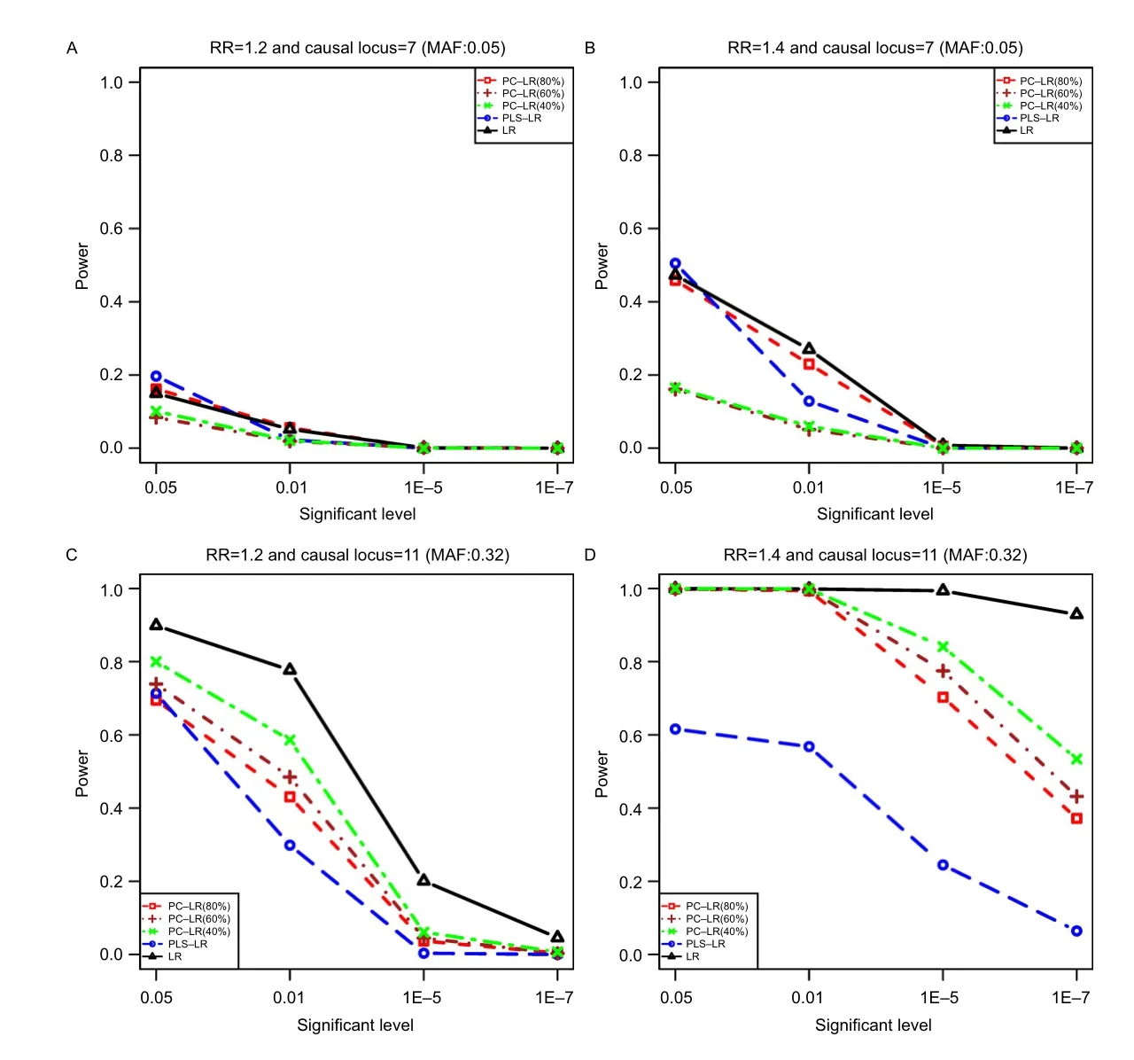
Fig.1The powers of principal component-based logistic regression(PC-LR),PLS logistic regression(PLS-LR)and single-locus logistic regression(LR)under different significant levels,relative risks(RR)and causal variants at the given sample size of 4,000.The horizontal axis(x-axis)denotes the significant level and the vertical axis(y-axis)denotes the powers of PC-LR(80%),PC-LR(60%),PC-LR (40%),PLS-LR and LR.Figure(A)and(B)depict the results obtained with the RR of 1.2 and 1.4 at the 7th loci,respectively;Figure(C)and(D)depict the results obtained with the RR of 1.2 and 1.4 at the 11th loci,respectively.

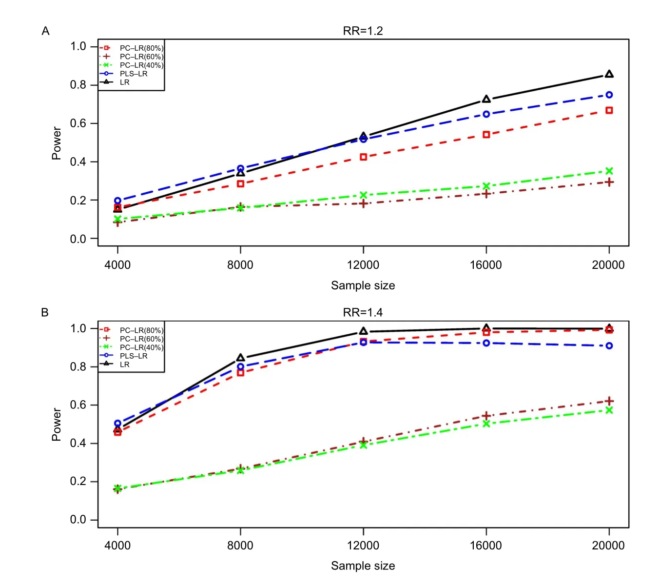
Fig.2The powers of principal component-based logistic regression(PC-LR),PLS logistic regression(PLS-LR)and single-locus logistic regression(LR)under different sample sizes at the given relative risk of 1.2 and 1.4 with the 7thSNP(rs6554759,MAF:0.053)on CLPTM1Lgene as the causal variant.The horizontal axis(x-axis)denotes the sample sizes and the vertical axis(y-axis)denotes the powers of PC-LR (80%),PC-LR(60%),PC-LR(40%),PLS-LR and LR.Figure(A)and(B)depict the results obtained with the RR of 1.2 and 1.4,respectively.

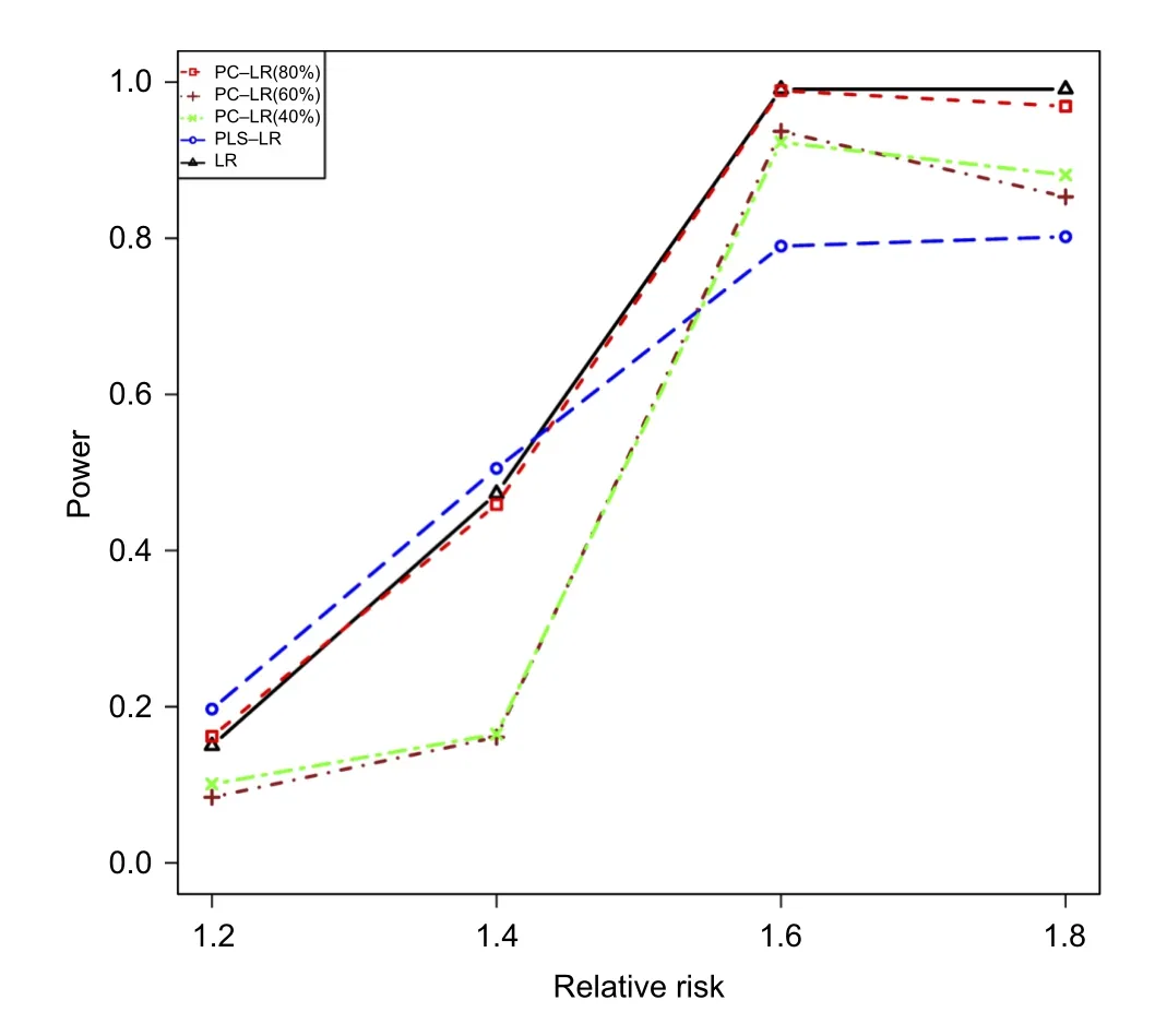
Fig.3The powers of principal component-based logistic regression(PC-LR),PLS logistic regression(PLS-LR)and single-locus logistic regression(LR)under different relative risks at the given sample size of 4,000 when the 7thSNP(rs6554759,MAF:0.053)on CLPTM1Lgene as the causal variant.The horizontal axis(x-axis)denotes the relative risks and the vertical axis(yaxis)denotes the powers of PC-LR(80%), PC-LR(60%),PC-LR(40%),PLS-LR and LR.

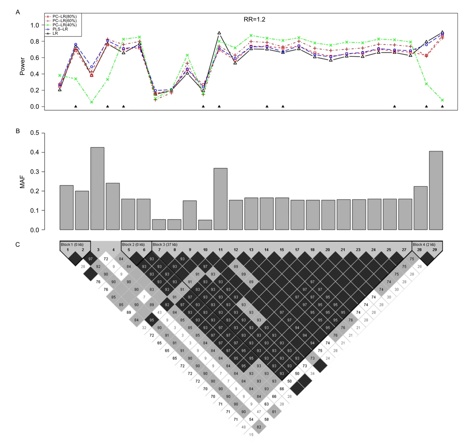
Fig.4The powers of principal component-based logistic regression(PC-LR),PLS logistic regression(PLS-LR)and single-locus logistic regression(LR)at the given sample size of 4000 and relative risk of 1.2 when each of the 25 SNPs was set as the causal variant based onCLPTM1Lgene.The top plot(A)shows the powers(y-axis)of PC-LR(80%),PC-LR(60%),PC-LR(40%),PLS-LR and LR over the positions(x-axis)of the causal SNPs.The triangles in the plot are the locations of the genotyped SNPs.The bar-plot in the middle panel(B) shows the MAFs of all SNPs.The pair-wise R2structure of the 25 SNPs is shown by the heat plot in the bottom of the figure(C),in which the gray scale indicates the value of R2(1=black,0=white).

Fig.5The SNP sets based analysis results of principal component-based logistic regression(PC-LR),PLS logistic regression (PLS-LR)and single-locus logistic regression(LR)on the MIPEP-TNFRSF19 gene region from the non-small cell lung cancer GWAS.The top plot(A)shows the p-values in-log10(p-value)scale(y-axis)of single-locus LR and SNPs sets based PC-LR over the locations(x-axis) of 21 SNPs.The haplotype block-based SNPs sets are showed as boxes on the top.For PC-LR method,the p-values of all SNPs in the same SNPs set are all denoted by the same p-value of the SNPs set.The bottom plot(B)shows the PLS-LR confidence intervals of standardized coefficients(y-axis)over the locations(x-axis)of 21 SNPs.★:significant at the level of 1E-6.

For region 2,the most highly ranked SNP was rs4488809(the 1stloci)from TP63 gene,with the least p-value of 2.61E-06 by single-locus LR.The p-value of PC-LR(40%)for the whole region was 1.51E-04.And the block 1 showed the least P-value(2.49E-06)of PC-LR among 16 SNPs sets.PLS-LR found that more locus showed the significance than other methods at the same level,including the 1st,38th,38th,41th,57th,63th,67thand 70thloci.

Discussion

High multicollinearity and multiple testing are major concerns for the analysis of GWAS[24-25]. Plenty of methods have been developed to overcome these problems[26-28].In recent years,dimension reduction-based methods,such as PCA and PLS,have been proposed to avoid the collinearity among SNPs,and reduce positive rate caused by multiple testing.Many studies suggested that utilizing the dimension reduction methods is effective in genetic association study[29-31].Chun et al.compared PLS regression with PC regression in the framework of linear regression for continuous response variables[32].However,in the case-control GWAS,the binary response variables are often used.In this situation,a logistic regression method in which the binary response is regressed on the PCs is used instead of linear model,such as PCLR and PLS-LR.

In this study,we propose to use PC-LR and PLS-LR as dimension reduction-based methods for the SNPs sets based analysis of case-control GWAS.We compare their performance with the single-locus analysis through extensive simulation studies using datasets generated from the International HapMap Project, and we also applied these two methods to two regions extracted form a real GWAS data on NSCLC.

In general,the simulation results demonstrate that all methods have type I error that is close to or lower than the nominal levels.Among all methods,PC-LR and PLS-LR perform well in terms of type I error under null hypothesis.In contrast,LR corrected by Bonferroni method is more conserved in all simulation settings.

In this study,the power of PC-LR is influenced by the MAF.When the MAF is relative rare(e.g.0.05), the power of PC-LR(40%)is the lowest among all methods(Fig.1).This may be due to the latent variable identified by the first few PCs that may be unrelated to outcome.It suggests that a few PCs that explain very little proportion of the total variation will lose power to detect genetic variants with lower MAF.

On the contrary,when the MAF of a causal allele is high(e.g.0.32),PC-LR(40%)is most powerful among all PC-LR methods(Fig.1).This may be due to the fact that when first a few PCs in the model have already explained the difference between cases and controls,including more PCs will not improve the model,but instead exhaust more degrees of freedom and decrease the test power slightly.

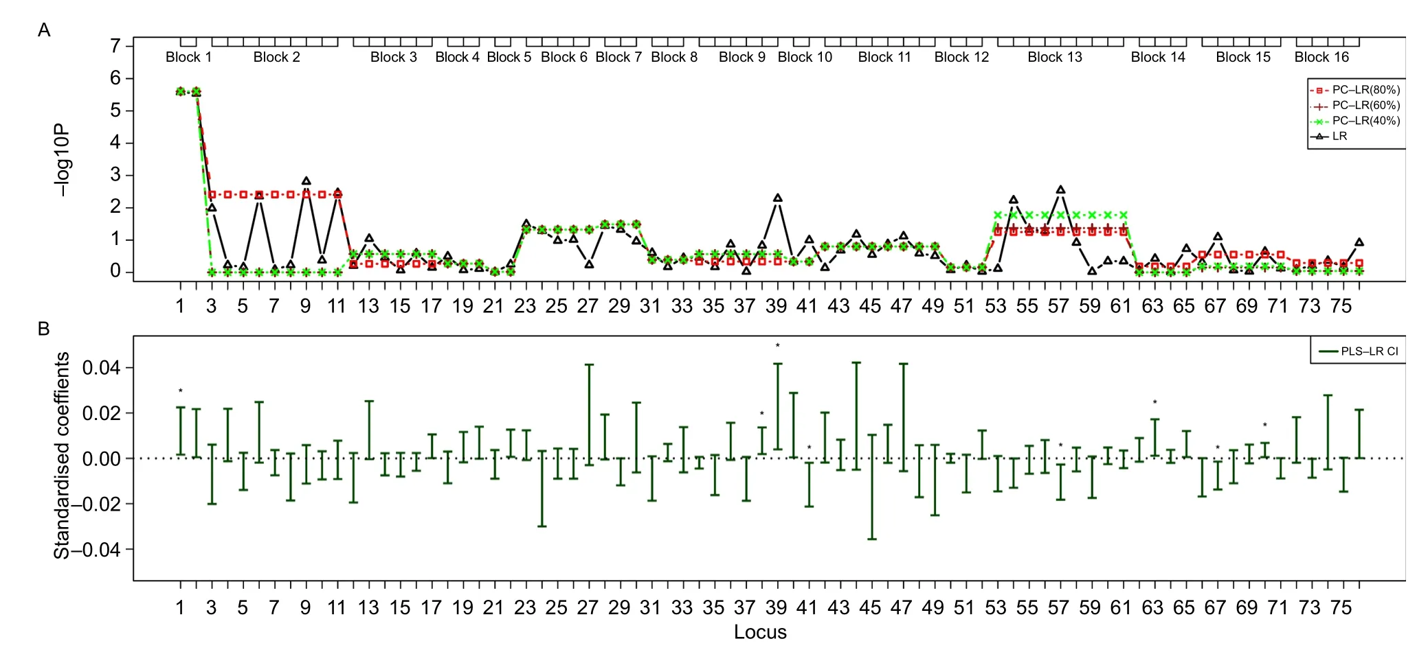
Fig.6The SNP sets based analysis results of principal component-based logistic regression(PC-LR),PLS logistic regression(PLS-LR) and single-locus logistic regression(LR)on the TP63 gene region from a non-small cell lung cancer GWAS.The top plot(A)shows the p-valuesin-log10(p-value)scale(y-axis)ofsingle-locusLRandSNPsetsbasedPC-LRoverthelocations(x-axis)of76SNPs.Thehaplotypeblock-basedSNPs setsareshowedasboxesonthetop.ForPC-LRmethod,p-valuesofallSNPsinthesameSNPssetarealldenotedbythesamep-valueoftheSNPsset.Thebottom plot(B)shows the PLS-LR confidence intervals of standardized coefficients(y-axis)over the locations(x-axis)of 76 SNPs.★:significant at the level of 1E-6.

Throughout the simulation study,the results suggest that without knowing the truth,no method always can identify the most associations in every scenario.However,PC-LR and PLS-LR perform better than LR when the causal SNP is in high LD with genotyped ones(Fig.4).This is because single-locus LR only utilizes one SNP in the analysis and there is no room to utilize the correlation among SNPs when doing so may boost the power.On contrast,PC-LR and PLS-LR are more powerful than LR at the strong LD locus,such as the causal loci at one of the 5th-6thand the 12th-27th.This demonstrates that PC-LR and PLS-LR have the ability of‘‘borrowing’’information to increase the statistical power based on LD.Therefore,we recommend the use of dimension reduction techniques,such as PC-LR or PLS-LR,in case-control GWAS.When the causal SNP is in poor LD with others and the cumulative contributing proportion of the total variability is 40%,the power of PC-LR decreased dramatically.Therefore,it is recommended by our results that a plenty of higher cumulative contributing proportion(such as 80%) can be used especially in a complex LD structure for PC-LR.

There are several limitations about our studies.Firstly, only one causal SNP is considered in the present simulation.Secondly,we find that PC-LR and PLS-LR have comparable power and they both outperform LR,especially in a small effective size(RR=1.2)and strong LD structure.However,PLS-LR is significantly slower than the other methods due to the bootstrap step.That may hamper the use of PLS-LR in real GWAS.Thirdly,more complicated situations,such as gene-gene interaction, goodness of fit and accuracy of parameter estimation of PLS,are not included in the study.Further investigations are needed to address these issues.

Acknowledgments

We thank all of the study subjects,research staff and students who participated in this work.We also appreciate the anonymous reviewers for their valuable suggestions for this manuscript.

[1] Altshuler D,Daly MJ,Lander ES.Genetic mapping in human disease[J].Science,2008,322(5903):881-888.

[2] Dichgans M,Malik R,Konig IR,et al.Shared genetic susceptibility to ischemic stroke and coronary artery disease: a genome-wide analysis of common variants[J].Stroke, 2014,45(1):24-36.

[3] Wang C,Xu Z,Jin G,et al.Genome-wide analysis of runs of homozygosity identifies new susceptibility regions of lung cancer in Han Chinese[J].J Biomed Res,2013,27(3): 208-214.

[4] Hill-Burns EM,Wissemann WT,Hamza TH,et al. Identification of a novel Parkinson’s disease locus via stratified genome-wide association study[J].BMC Genomics, 2014,15(1):118.

[5] Moskvina V,Harold D,Russo G,et al.Analysis of genome-wide association studies of Alzheimer disease and of Parkinson disease to determine if these 2 diseases share a common genetic risk[J].JAMA Neurol,2013,70(10): 1268-1276.

[6] Hu Z,Wu C,Shi Y,et al.A genome-wide association study identifies two new lung cancer susceptibility loci at 13q12.12 and 22q12.2 in Han Chinese[J].Nat Genet, 2011,43(8):792-796.

[7] Hu Z,Shi Y,Mo X,et al.A genome-wide association study identifies two risk loci for congenital heart malformations in Han Chinese populations[J].Nat Genet, 2013,45(7):818-821.

[8] Ward LD,Kellis M.Interpreting noncoding genetic variation in complex traits and human disease[J].Nat Biotechnol,2012,30(11):1095-1106.

[9] Moore JH,Asselbergs FW,Williams SM.Bioinformatics challenges for genome-wide association studies[J]. Bioinformatics,2010,26(4):445-455.

[10]Beyene J,Tritchler D,Asimit JL,et al.Gene-or regionbased analysis of genome-wide association studies[J]. Genet Epidemiol,2009,33(S1):S105-S110.

[11]Zhao Y,Chen F,Zhai R,et al.Association test based on SNP set:logistic kernel machine based test vs.principal component analysis[J].PLoS One,2012,7(9):e44978.

[12]Gauderman WJ,Murcray C,Gilliland F,et al.Testing association between disease and multiple SNPs in a candidate gene[J].Genet Epidemiol,2007,31(5):383-395.

[13]Rosipal R,Kra¨mer N.Overview and Recent Advances in Partial Least Squares.In::Saunders C,Grobelnik M, Gunn S,Shawe-Taylor J,Editors.Subspace,Latent Structure and Feature Selection,New York:Springer Berlin Heidelberg,2006:34-51.

[14]Chun H,Keles S.Sparse partial least squares regression for simultaneous dimension reduction and variable selection[J].Journal of the Royal Statistical Society: Series B(Statistical Methodology),2010,72(1):3-25.

[15]Marx BD.Iteratively Reweighted Partial Least Squares Estimation for Generalized Linear Regression[J]. Technometrics,1996,38(4):374-381.

[16]Bastien P,Vinzi VE,Tenenhaus M.PLS generalised linear regression[J].Computational Statistics&Data Analysis,2005,48(1):17-46.

[17]Boulesteix AL,Strimmer K.Partial least squares:a versatile tool for the analysis of high-dimensional genomic data[J].Brief Bioinform,2007,8(1):32-44.

[18]Fort G,Lambert-Lacroix S.Classification using partial least squares with penalized logistic regression[J].Bioinformatics,2005,21(7):1104-1111.

[19]Nygard S,Borgan Ø,Lingjærde O,Størvold H.Partial least squares Cox regression for genome-wide data[J]. Lifetime Data Analysis,2008,14(2):179-195.

[20]Chun H,Ballard DH,Cho J,et al.Identification of association between disease and multiple markers via sparse partial least-squares regression[J].Genetic Epidemiology, 2011,35(6):479-486.

[21]SuZ,MarchiniJ,DonnellyP.HAPGEN2:simulationofmultiple disease SNPs[J].Bioinformatics,2011,27(16):2304-2305.

[22]Barrett JC,Fry B,Maller J,Daly MJ.Haploview:analysis and visualization of LD and haplotype maps[J]. Bioinformatics,2005,21(2):263-265.

[23]Miki D,Kubo M,Takahashi A,et al.Variation in TP63 is associated with lung adenocarcinoma susceptibility in Japanese and Korean populations[J].Nat Genet, 2010,42(10):893-896.

[24]Hayes B.Overview of Statistical Methods for Genome-Wide Association Studies(GWAS)[J].Methods Mol Biol,2013,1019:149-169.

[25]Watanabe RM.Statistical issues in gene association studies[J].Methods Mol Biol,2011,700:17-36.

[26]He Q,Lin DY.A variable selection method for genomewide association studies[J].Bioinformatics,2011,27(1): 1-8.

[27]Fridley BL,Biernacka JM.Gene set analysis of SNP data: benefits,challenges,and future directions[J].Eur J Hum Genet,2011,19(8):837-843.

[28]Wang X,Morris NJ,Schaid DJ,et al.Power of Single-vs. Multi-Marker Tests of Association[J].Genetic Epidemiology,2012,36(5):480-487.

[29]Wang T,Ho G,Ye K,et al.A partial least-square approach for modeling gene-gene and gene-environment interactions when multiple markers are genotyped[J]. Genet Epidemiol,2009,33(1):6-15.

[30]Chen X,Wang L,Hu B,et al.Pathway-based analysis for genome-wide association studies using supervised principal components[J].Genet Epidemiol,2010,34(7):716-724.

[31]Mei H,Chen W,Dellinger A,He J,Wang M,Yau C,et al. Principal-component-based multivariate regression for genetic association studies of metabolic syndrome components[J].BMC Genet,2010,11:100.

[32]Chun H,Ballard DH,Cho J,et al.Identification of association between disease and multiple markers via sparse partial least-squares regression[J].Genet Epidemiol,2011; 35(6):479-486.

This work wasfounded by the NationalNaturalScience Foundation ofChina(81202283,81473070,81373102 and 81202267),Key Grant of Natural Science Foundation of the Jiangsu Higher Education Institutions of China(10KJA330034 and 11KJA330001),the Research Fund for the Doctoral Program ofHigherEducation ofChina (20113234110002)and the Priority AcademicProgram fortheDevelopmentofJiangsu HigherEducation Institutions(Public Health and Preventive Medicine).

△These authors contributed equally to this work.

✉Corresponding author:Prof.Feng Chen,Department of Epidemiology and Biostatistics,School of Public Health,Nanjing Medical University, Nanjing,Jiangsu 211166,China.Tel:+86-25-86868414,E-mail: fengchen@njmu.edu.cn.

Received 11 March 2014,Revised 29 September 2014,Accepted 15 January 2015,Epub 20 April 2015

R181.2,Document code:A

The authors reported no conflict of interests.