
Numerical Simulation of Strong Shock Wave Impacting on Water-elastic Solid Interface by Essentially Modified Ghost Fluid Method
2015-12-12 08:52:42SHIRuchaoWANGGuangyongHUANGRuiyuanWANGYoukaiLIYongchi
船舶力学 2015年9期
SHI Ru-chao,WANG Guang-yong,HUANG Rui-yuan,WANG You-kai,LI Yong-chi
(1.School of Civil Engineering,Henan Polytechnic University,Jiaozuo 454000,China;2.Department of Modern Mechanics,University of Science and Technology of China,Hefei 230027,China)
0 Introduction
Strong shock wave impacting on water-elastic solid interface is still a hot area of research in computational physics and engineering problems.For computational physics,solid is assumed or treated as elastic to develop novel computational method for fluid-structure interaction[6,9,16]or to simplify complicated problems to obtain high quality graphics[2].On the other side of application,in engineering problem such as underwater explosion and impact dynamics,solid is also constantly assumed to be elastic to provide comparisons with experimental results[7,10].
The original Ghost Fluid Method(OGFM)developed by Fedkiw and Aslam et al[5]and some improved methods have been widely applied for simulating multi-medium flow.The OGFM is able to work efficiently for gas-gas flow and gas-water flow with low ratio of pressure on material interface.Improved GFMs include new version GFM(NGFM)[6],modified GFM(MGFM)[13]and real GFM(RGFM)[21].Among these three methods,NGFM is designed for fluid-structure interaction and also can be applied for gas-water flow,and MGFM which is the most popular method has been found to be not only quite competent to simulate fluid-fluid interface with high ratio of interface but also capable to simulate propagation of shock wave in solid(essentially MGFM)[16-17]by combining with Naviers equation[4],and RGFM can be used to treat extreme and special situation.
In this work,we employ the idea of essentially MGFM to simulate strong shock wave impacting on water-solid interface while fundamental elastodynmaics equations and the constitutive relationship of linear elastic are used to solve solid.The following text is arranged as follows.In Chapter 1,we present governing equations and EOS.Then,the approximate Riemann problem relationship for water-elastic solid are presented in Chapter 2.Next,we present numerical results with the employment of essentially MGFM in Chapter 3.And some summarizations and conclusions are given briefly in last Chapter.
1 Governing equations
1.1 Euler equations
The flow field of water is solved by Euler equations:
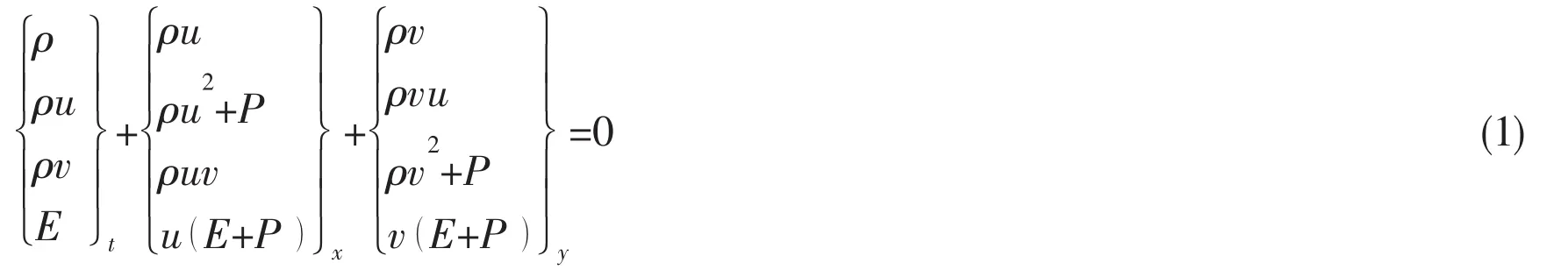
where ρ is density,u and v are velocities at x and y directions,respectively.is total energy.Here,e is internal energy per unit mass.Euler equations are solved with fifthorder WENO spatial discretization[17]and second-order Runge-Kutta(R-K)time discretization.The stability condition is CFL≤1.
1.2 Fundamental elastodynamics equations
The constitutive relationship of elastic solid is Hooke’s law which can be expressed as

where ε represents the strain,E is Young’s Modulus and σ is stress.In general,the tensile stress of solid is defined as positive.We use fundamental elastodynamics equations[12]to solve elastic solid.For 1D problem,continuity equation is

and the momentum equation is

For multi-dimensional problems,the governing equations are given as

where
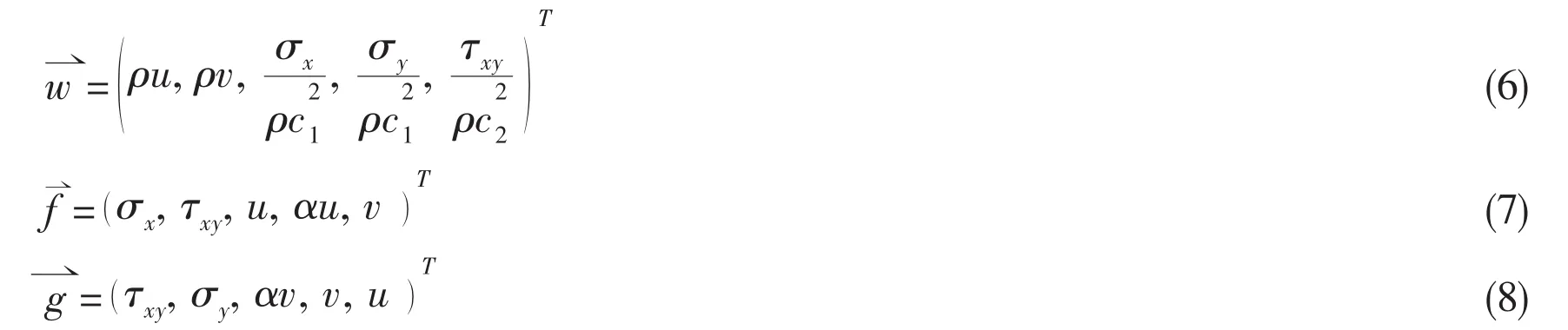
where ρ is the constant solid density,c1and c2are velocities of longitudinal wave and shear wave,respectively.Generally,α=1-2(c2/ c1)2for isotropic materials,and c1,c2can be expressed as:
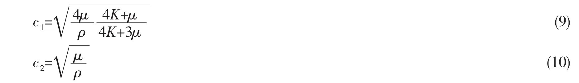
where K=E/[3(1-2μ)]is bulk modulus and μ is Poisson’s ratio.In the test of Chapter 3,fundamental elatodynamics equations are discretized by bicharacteristic schemes[11].The stability condition is max(Δx/Δt,Δy/Δt)≤1/c1.In calculations,Δt should satisfy both solid stability condition and fluid stability condition(CFL≤1).
1.3 Equations of state
For gas,the EOS is γ-law,

For water,Tait equation[20]and isentropic one-fluid model[14]are employed here and can be given as
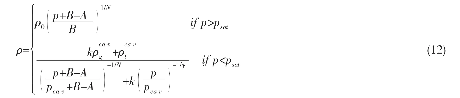
where psatis the saturated pressure of water,N=7.15,γ=1.33,ρ0=1.0×10³kg/m3,B=3.31×108Pa and A=1.0×10⁵Pa,pcav=psat,the initial value of k is set to be k=0.001 and k should be updated by knew=0.9k if the result of p is beyond psat.For steel,the density is constant and set to be 7.8×10³kg/m3,Young’s modulus E=2.06×10¹¹Pa,Poisson’s ratio μ=0.25.
1.4 Level set method
For Eulerain grids of fluid,we use Level set equation[18]to keep track of material interface,

where φ is signed distance function.For Lagrangian grids of solid,we transform Level set equation from the local coordinates into the arbitrary coordinates(ξ,η),

Eqs.(13)and(14)are solved with fifth-order HJ-WENO spatial discretization[8]and secondorder R-K time discretization.For Eq.(14),ξx,ξy,ηx,ηyare solved via grid derivatives xξ,xη,yξ,yηand the relationship of coordinate transformation.The grid derivatives are discretized by second-order central difference in entire domain and second-order upwind difference at boundary.
The extension velocity method[1]is employed to improve the accuracy of Level set method while tracking material interface.For Eulerian grids,extension velocity is expressed as

where the vector vextis the extension of velocities at the grid nodes bordering material interface.For Lagrangian grids,▽φ and▽vextin Eq.(15)should be written as

and

In calculations,▽φ is discretized by fifth-order HJ-WENO scheme and▽vextis discretized by first-order MinMod upwind scheme.
1.5 Constant extrapolation
For Eulerian grids,we use the constant extrapolation method in Refs.[3,5],which can be given as

where I is the function that need to be extrapolated,nxand nyare components of interfacial unit normal vector n that can be expressed as

For Eq.(18),the sign‘ ±’is taken as‘+’if the initial values of I is defined in Ω-and need to be extrapolated into Ω+.Otherwise,the sign ± is taken as‘-’.For Lagrangian grids,we need to transform the constant extrapolation equation from the local coordinates into the arbitrary coordinates(ξ,η).Hence Eq.(18)should be rewritten as

In Eqs.(18)-(20),nxand nyare determined by▽φ which is given as Eq.(16).
2 Essentially MGFM for fluid-elastic solid interface
2.1 Approximate Riemann problems solver
Defining the tensile stress of solid as negative to maintain the same sign as the pressure of fluid,we can rewrite Eqs.(3)and(4)as:

and

We might suppose that fluid is on the left side of fluid-solid interface while solid is on the right side of fluid-solid interface.On the side of fluid,the characteristic equation along the right characteristic line is

where p1and uIare the pressure and velocity at interface,ρILand cILare the left density and sound velocity in the immediate vicinity of interface.On the right side of interface,the characteristic equation alongside left characteristic line can be given as

where σIand uIare the stress and velocity at interface,ρRand ERare the density and Young’s modulus of the medium on the right side of interface.For Eq.(23),we can use WILto approximate ρc,which is given as[13]
ILIL

Then,Eqs.(23)with(24)reveal the following equations:
Noting that the intial stress of solid is equal to gauge pressure,σIshould be defined as

where penvdenotes the environment pressure.
2.2 Numerical implementation
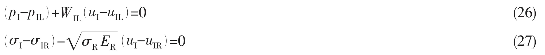
In calculations,the region of fluid is discretized by Eulerian grids while the region of solid is discretized by Lagrangian grids.For the grid nodes of fluid,we define the grid nodes as real if there is medium of fluid at those grid nodes,otherwise,we define those grid nodes as ghost.We treat the grids nodes of solid in the similar way.At every computational time step,the locations of solid medium are recorded by the coordinates of Lagrangian grid nodes to track solid boundary and fluid-solid interface.The schematics of the MGFM algorithm is shown as Fig.1 and computational procedures are summarized as follows:
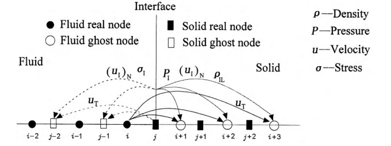
Fig.1 Schematics of MGFM for treating fluid-elastic solid coupling
(1)Respectively divide the nodal points in Eulerian grids of fluid and in Lagrangian grids of solid into real nodal points and ghost nodal points according to the location of fluid-solid interface.
(2)Identify the interfacial cells for both the Eulerian grids and Lagrangian grids and seek out a real nodal point x in Lagrangian grid of solid to define one-dimensional Riemann problems for every real nodal points xmEulerian grid of fluid using the employment of minimum angle algorithm which can be expressed as

(3)Solve the interfacial status via Eqs.(25)-(28)for every one-dimensional Riemann problem in step(2).
(4)Extrapolate the interfacial status(ρIL,pIand uI)and left tangential velocity(uT)from real region of fluid into ghost region of fluid.
(5)Solve all nodal points of Eulerian grids of fluid.
(6)Seek out a real nodal point x in Eulerian grid of fluid to define one-dimensional Riemann problems for every real nodal points xmin Lagrangian grid of solid.
(7)Solve the interfacial status via Eqs.(25)-(28)for every one-dimensional Riemann problem in step(6).
(8)Extrapolate the interfacial status(σIand uI)and right tangential velocity(uT)from real region of solid into ghost region of solid in Lagrangian solid.
(9)Solve all nodal points in Lagrangian grids of solid.
(10)Keep track of fluid-solid interface by Level set method in Lagrangian grid of solid while the boundary of solid is always set to be fluid-solid interface at every computational time step,which can be expressed as φ(solid boundary)=0.
(11)Update the φ values at Eulerian grid nodes of fluid and update the status at real nodal points of both Eulerian and Lagrangian grids by the location of fluid-solid interface.
3 Numerical results
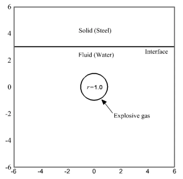
Fig.2 Schematics of the initial computational region
The numerical example is a case of column charge underwater explosion near a planar elastic solid(steel).The reason why we use this case is that underwater explosion can generate strong shock wave impacting on fluid-solid interface and then results a strong reflection wave from fluid-solid interface.The radius and density of column charge is 1.0m and 1 270.0 kg/m3,respectively.The problem can be cast into 2D system and the result has already been presented in Ref.[15]by compressible solid assumption which means that the solid is assumed to be compressible when the shock wave generated by underwater explosion impacting on fluid-solid interface.The feasibility of this assumption was also verified in Ref.[22]using large amounts of tests.In this test,the assumption of elastic solid is employed and the feasibility has been verified in Ref.[16]and[17].Following the idea in Ref.[15],we employ instantaneous detonation model to treat detonation product as high energy gas,since it is not necessary to use other more complicated model to treat detonation product when we only need to test the performance of Riemann relationship developed as applied to fluid-solid interface.Consequently the detonation product becomes a high pressure bubble at the initial computational time.The numerical simulation is accomplished by the presented model of fluid-solid interaction and the MGFM model of gas-water interaction in Ref.[13].The related detonation parameters and the corresponding initial computational flow states are taken directly from Ref.[15].The initial pressure of high pressure bubble is pg=8 290.0 bar which is equal to the multiplication of equivalent coefficient α and detonation pressure pCJ.The initial density is ρg=1 270.0 kg/m3which is equal to the charge density.The explosive gas satisfies EOS of γ-law where γg=2.0 which were obtained in experiments.The initial status of water is pw=1.0 bar,ρw=1 000.0 kg/m3,the density of solid is ρs=7 800.0 kg/m3and penvin Eq.(28)is set to be 1.0 bar.As shown in Fig.2,the high pressure bubble under water is initially located in the origin(0,0)of Cartesian coordinates and the radius is 1.0 m,and the eleastic solid is located at the straight line y=3 m.As shown in Fig.3,The computational region of fluid is[-6 m,6 m]×[-6 m,4 m]with 121×101 uniform grid nodes distributed and the initial computational region of solid is[-6 m,6 m]×[2 m,6 m]and discretized by 121×41 uniform grid nodes.In calculations,an arbitrary coordinate system is constructed for Lagrangian grids of solid.
Fig.3 The computational region of fluid and solid.(a)Fluid,(b)Solid
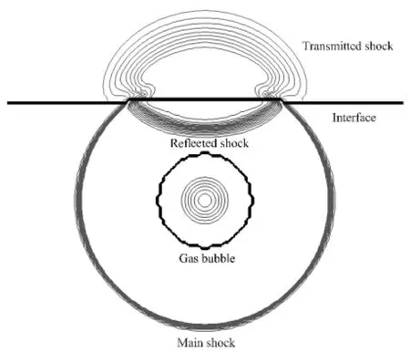
Fig.4 Pressure contours at t=1.47 ms
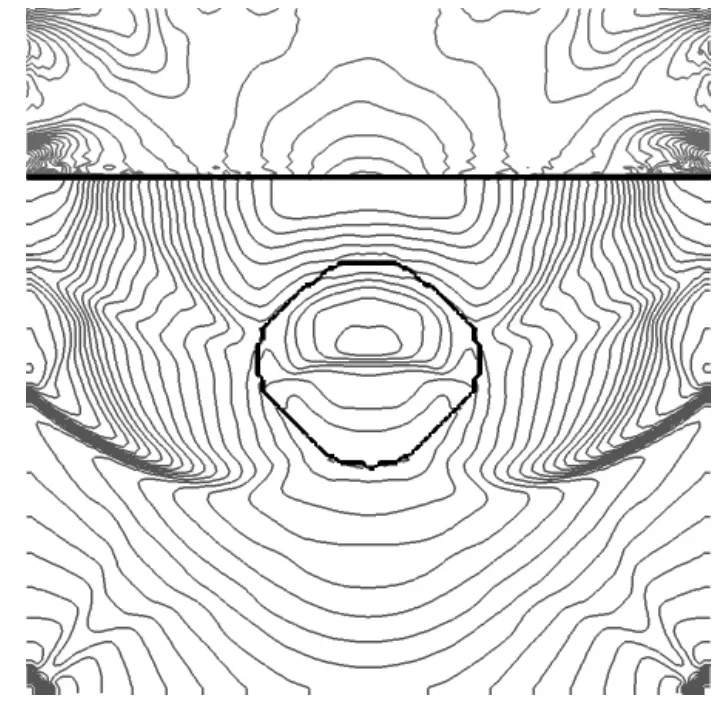
Fig.5 Pressure contours at t=3.99 ms
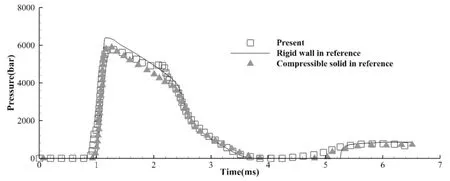
Fig.6 Comparisons among the results on elastic solid,compressible solid and rigid wall
Once the explosion starts,a strong shock wave is generated and propagates outwards to fluid-solid interface.Series of pressure contours at t=1.47 ms are depicted in Fig.4 where the pressure of solid is hydrostatic pressure,which can be expressed as ps=(σx+σy)/3.The transmitted shock propagating in elastic solid is captured and shown in Fig.5.There are some differences between the numerical results presented here and in Ref.[15].The reason is that the solid is compressible in Ref.[15]but incompressible in this case.Since the constitutive relation is linear elastic,the fluid-solid interface compressed by incident shock gradually return to original shape as the pressure at the wall center decreases and to tend to near zero.To better verify the numerical results and display the differences between the assumption of elastic solid,compressible solid and rigid wall,the pressure loads at the center of wall are recorded and depicted in Fig.6.The numerical results on assuming that solid is rigid wall and compressible solid are taken directly form Ref.[15].In Fig.6,the peak pressure presented is similar to the result by compressible solid assumption.Both the peak pressures by these two different assumptions are below the result by rigid wall.Fig.6 also demonstrates that the times of different assumption,when the cavitation occurs,are very close to each other.
4 Conclusions
In this work,we present a Riemann relationship for fluid-elastic solid interface and employ the idea of essentially MGFM to treat fluid-elastic solid interaction.The Level set equations in Lagragian grids are also presented by employing the transformation between Cartesian coordinates and arbitrary coordinates.We compare the results on strong shock wave impacting on rigid wall,compressible solid and elastic solid.Numerical results demonstrate that the presented method is robust and efficient as applied for computing shock loading on fluid-elastic solid interface and works successfully on capturing reflection wave from material interface and the stress wave in solid.
[1]Adalsteinsson D,Sethian J.The fast construction of extension velocities in level set methods[J].J Comput.Phys.,1999,148:2-22.
[2]Aivazis M,Goddard W,Meiron D,et al.A virtual test facility for simulating the dynamic response of materials[J].Comput in Sci.and Eng.,2000,2:42-53.
[3]Aslam T.A partial differential equation approach to multidimensional extrapolation[J].J Comput.Phys.,2004,193:349-355.
[4]Chung T J.Applied continuum mechanics[M].Cambridge University Press,New York,1996.
[5]Fedkiw R,Aslam T,Merriman B,et al.A non-oscillatory Eulerian approach to interfaces in multimaterial flows(the ghost fluid method)[J].J Comput.Phys.,1999,152:457-492.
[6]Fedkiw R.Coupling an Eulerian fluid calculation to a Lagrangian solid calculation with the ghost fluid method[J].J Comput.Phys.,2002,175:200-224.
[7]Greco M,Colicchio G,Faltinsen O M.A domain-decomposition strategy for a compressible multi-phase flow interacting with a structure[J].International Journal for Numerical Methods in Engineering,2014,98:840-858.
[8]Jiang G S,Peng D.Weighted ENO schemes for Hamilton Jacobi equations[J].SIAM J Sci.Comput.,2000,21:2126-2143.
[9]Kaboudian A,Khoo B C.The ghost solid method for the elastic solid-solid interface[J].Journal of Computational Physics,2014,257:102-125.
[10]Li Qinyuan,Manolidis Michail,Young Yin L.Analytical modeling of the underwater shock response of rigid and elastic plates near a solid boundary[J].Journal of Applied Mechanics-Transactions of the ASME,2013,80:2.
[11]Lin X,Ballman J.Improved bicharacteristic schemes for two-dimensional elastody-namic equations[J].Quarterly of Applied Mathematics,1995,53:383-398.
[12]Lin X.Numerical computation of stress waves in solid[M].Akademie,Berlin,1997.
[13]Liu T G,Khoo B C,Yeo K S.Ghost fluid method for strong shock impacting on material interface[J].J Comput.Phys.,2003,190:651-681.
[14]Liu T G,Khoo B C,Xie W F.Isentropic one-fluid modelling of unsteady cavitating flow[J].J Comput.Phys.,2004,201:80-108.
[15]Liu T G,Khoo B C,Xie W F.The modified ghost fluid method as applied to extreme fluid-Structure interaction in the presence of cavitation[J].Communication in Computational Physics,2006,1:898-919.
[16]Liu T G,Ho J Y,Khoo B C,et al.Numerical simulation of fluid-structure interaction using modified ghost fluid method and Naviers equations[J].J Sci.Comput.,2008,36:45-68.
[17]Liu T G,Chowdhury A W,Khoo B C.The Modified Ghost Fluid Method applied to fluid-structure interaction[J].Advances in Applied Mathematics and Mechanics,2011,3:611-632.
[18]Osher S,Sethian J A.Fronts propagating with curvature-dependent speed:Algorithms Based on Hamilton-Jacobi Formulations[J].J Comput.Phys.,1988,79:12-49.
[19]Shu C W.Essentially non-oscillatory and weighted essentially non-oscillatory schemes for hyperbolic conservation laws[R].ICASE Report No.97-65,1997.
[20]Wardlaw A.Underwater explosion test cases[R].IHTR-2069,1998.
[21]Wang C W,Liu T G,Khoo B C.A real ghost fluid method for the simulation of multimedium compressible flow[J].SIAM J Sci.Comput.,2005,128:278-232.
[22]Xie W F,Young Y L,Liu T G.Multiphase modeling of dynamic fluid-structure interaction during close-in explosion[J].Int.J Numer.Meth.Engng,2008,74:1019-1043.

- 船舶力学的其它文章
- Study of Damping Ratio Identification for a Truss Spar Based on Continuous Wavelet Transform
- Study on Vortex Induced Characteristics of Four Square Columns at Different Spacing Ratio
- Roll Motion Prediction of PSV with Anti-rolling Tank Based on RANS and Nonlinear Dynamic Method
- A Double-layer Depth-averaged Boussinesq Model for Water Wave
- Fatigue Strength Evaluation of Transverse Fillet Welded Joints Based on Notch Stress Strength Theory
- Low Noise Collocation on Fluid Pipeline System