A general framework for verification and validation of large eddy simulations＊

XING Tao

Department of Mechanical Engineering, College of Engineering, University of Idaho, Moscow, Idaho 83844,USA, E-mail: xing@uidaho.edu

Introduction

With the dramatic increase and growth of supercomputers, simulation based design, and ultimately virtual reality, have become increasingly important as means to take advantage of increased computing power for the advancement of science and engineering practice. Computational fluid dynamics (CFD) provides computerized solutions for science and engineering problems using mathematical physics modeling,numerical methods, and high performance computing.Mathematical physics modeling is in the form of continuous partial differential equations with appropriate boundary conditions and initial conditions. The continuous partial differential equations must be discretized into algebraic equations using numerical methods.The algebraic equations are assembled and solved to get approximate solutions. Simulation based design using CFD is widely accepted and used in industrial applications. Numerical benchmarks have become the standard for design in industrial applications, such as the vital role of CFD in the development of nearly all Boeing products[1], computational ship hydrodynamics[2], and offshore wind turbines[3-5]. CFD will not completely replace analytical methods and experimental measurements, but can provide the third approach to interpret flow physics, design fluid systems, and help understand physical fluid phenomena that are difficult or impossible to explain through experiments and theory. CFD can be used as a design tool and help improve the design for experiments. Recently, researchers have performed large-scale CFD simulations using hundreds of millions or even billions of grid points (Fig.1).

Selection of CFD models is mainly determined by flow regime, target accuracy, and available computational resources. Direct numerical simulation (DNS)solves the Navier-Stokes (N-S) equations without using a turbulence model. All the length scales of the flow must be resolved in the mesh. The total number of grid points increases asThus, DNS is mainly used as a fundamental research tool for understanding flow physics at low or moderate Reynolds numbers (Re). For highRe, turbulence models are needed such as Reynolds-averaged Navier-Stokes(RANS), large eddy simulation (LES), and hybrid RANS/LES. LES solves spatially filtered N-S equations such that large scales of the flow field are better resolved than RANS and the smallest and most expensive scales of the solution are modeled using sub-grid scale (SGS) models[6]. Recent studies have shown that LES provides a tractable method for the simulation of turbulent flows at highRein complex geometries[7-10].Unlike the weak grid sensitivity for RANS models[11],LES belongs to the category of multiscale models that resolve different flow physics at different length scales. Thus, LES resolves smaller and smaller length scales as the mesh is refined. When the mesh is the same as a DNS mesh, the LES should obtain the same solution as the filtered DNS results.

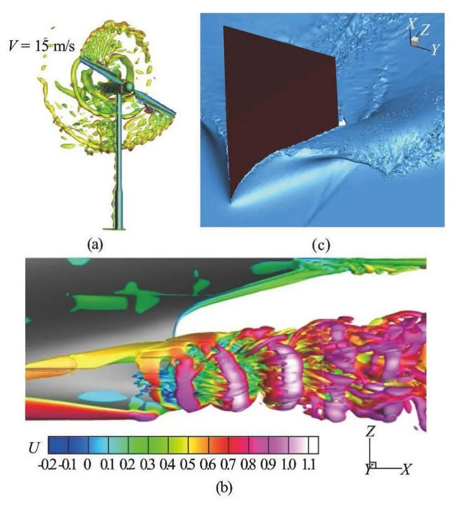
Fig.1 Samples of recent large-scale CFD simulations: (a) Detached Eddy Simulation (DES) for onshore wind turbine on a 53M grid[12], (b) DES of flow around a tanker on a 305M grid[11], and (c) DNS of water and air flows around a wedge using 2 billion grid points[13]

With the rapid increase of using CFD for academic research and industrial innovation, it is imperative to quantitatively estimate the numerical and modeling errors and associated uncertainties, which will provide guidelines for estimating the risk and reliability of the simulation based designs. Additionally, guidelines for how to optimize a CFD simulation to obtain a minimum total simulation error are needed. The approximation used in CFD will result in the simulation errorsδ, which is the difference between a simulation valueSand the truthT.

Since the true values of simulation quantities are rarely known, errors must be estimated. An uncertaintyUis an estimate of an error such that the interval ofU, ±U, bounds the true value ofsδ95 times out of 100, i.e., at the 95% confidence level for CFD[14].An uncertainty interval thus indicates the range of likely magnitudes ofsδbut no information about its sign.

1. Previous research on verification and validation and limitations

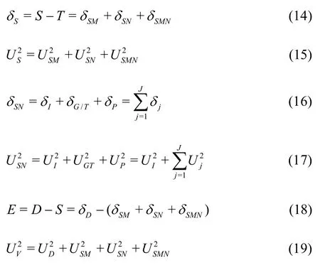
Existing V&V methods for CFD are mainly derived for RANS where the sources of errors and uncertainties for simulations can be divided into two distinct sources: modeling and numerical. Solution verification, which is a process for assessing numerical errorsδSNand uncertaintiesUSN. It is postulated that the simulation error and the corresponding simulation uncertaintyUScan be estimated using the following two equations, respectively[15]:

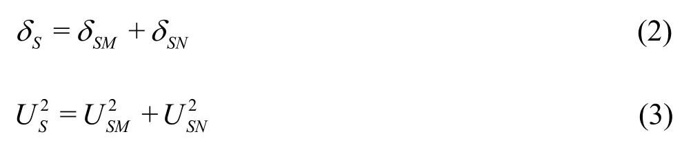
Validation is a process for assessing modeling uncertaintyUSMusing benchmark experimental dataD.

whereEis the comparison error,=D-Tis the difference between experimental data and the truth,andis the validation uncertainty. When,the model is validated[15,16]. Various methodology and procedures have been proposed for estimatingδSNand, including variants of the grid convergence index (GCI) method[17-21], correction factor method[15,22,23], factor of safety (FS) method[24,25], singlegrid method[26], and variants of the least-square method[27-29]. The FS method was recently evaluated as a method that can be applied successfully for accurate uncertainty estimation[30].

The existing V&V methods for RANS have at least two of the following limitations: (1) they either do not de-couple the numerical and modeling errors or ignore the coupling between numerical and modeling errors and thus cannot be used directly for LES, (2)the uncertainty as a result of modeling errors is not considered in the validation uncertainty, (3) they require the knowledge ofthat cannot be determinedwhen mixed numerical methods are used[31], (4) UVexcludes the uncertainty as a result of modeling assumptions[32]and (5) except the FS method, they lack statistical analysis to prove the achievement of 95%confidence level.

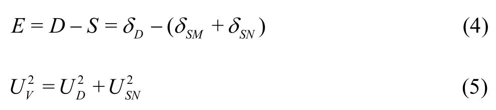
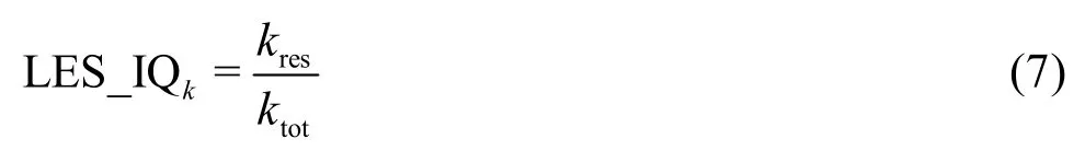
In order to quantify the “distance” between a particular LES and DNS, a few indices have been developed as single-grid estimators, including the “subgridactivity” parameter s[33,34]that measures the relative subgrid-model dissipation rate, modified activity parameters s*[35], relative Kolmogorov scale index LES_IQη[35], the relative sgs-viscosity index LES_IQν[35]and the relative resolved turbulent kinetic energy (TKE) content

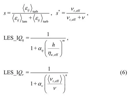
The use of the above formulas is difficult as all of them have at least one parameter that is difficult to estimate and must be approximated using empirical equations[36]. Additionally, some parameters (e.g., m and n) should be functions of Re but no explicit formulations are available. An alternative method is to use the resolved turbulent kinetic energy kresversus the total ktot

Celik et al.[35]proposed various ways to estimatedepending on how ktotis calculated. Five calculations will be needed if it is postulated thatIf the filter width Δ is equal to a constant times the grid spacing h and p=q, thenand only three calculations on three grids are needed. If p=2 is further assumed, then a two-grid estimator is obtained. These indices don’t explicitly elucidate the numerical and modeling errors and uncertainties.

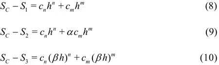
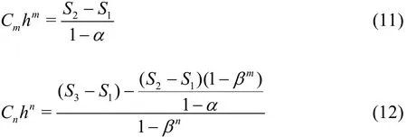
Rigorous assessment of the quality and reliability of LES simulations must be conducted using a systematic grid and model variation of influencing parameters (e.g., filter width and grid spacing). Klein[37]and Freitag and Klein[38]assumed that the contributions from the numerical error (n) and modeling error (m)are given by the right-hand side of the Taylor expansion, Eq.(8), where SCis the numerical benchmark.Changing the model contribution by a certain factor α and changing the grid spacing by a certain factor β yield Eqs.(9) and (10), respectively.

The uncertainty was evaluated using

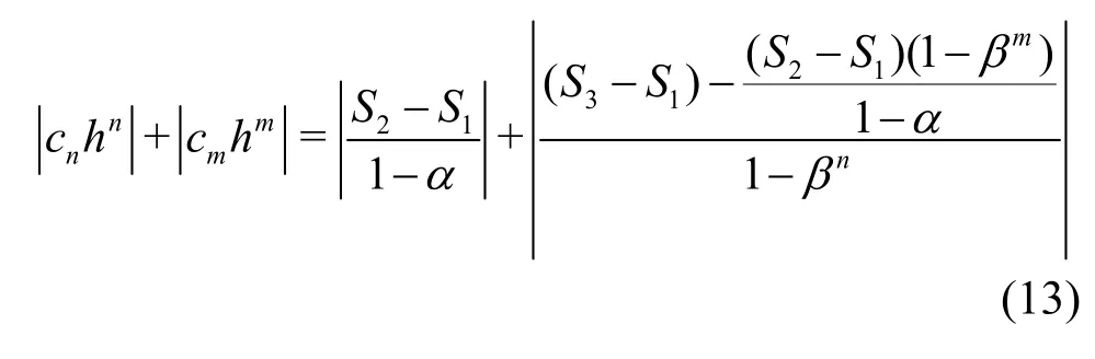
This method has some limitations: (1) numerical error due to temporal discretization and the coupling error between the numerical and modeling are neglected, (2)the formula for uncertainty estimation is not validated and does not include any factors of safety, (3) it cannot be used for explicitly filtered LES because the filter width is assumed to be the same as the grid spacing,(4) it does not consider the circumstances that the numerical and modeling errors have different signs and cancel each other out[35], and (5) n must be assumed to be equal to the theoretical (nominal) order of accuracy of the numerical scheme and m is a function of Re without specific guidelines.

2. Objective

Application of LES has been severely limited dueto lack of a general framework for quantitatively estimating errors and uncertainties for LES models. This is partially because of the nonlinear coupling between numerical and modeling errors. It has been observed by some studies that LES on a finer grid yields results with a large total error[39,40]. So, instead of always achieving more accurate solutions on finer grids typically observed for RANS models, the total error for LES arises from a balance between the numerical and modeling errors due to the counteracting property of the errors and their specific reverse dependence on filter width[39].

The urgent need for LES V&V has been recognized by the CFD community. Sagaut and Deck[41]pointed out for status and perspectives of LES for aerodynamics, “a clear need for detailed validation in the near future is identified. To this end, new issues, such as uncertainty and error quantification and modeling,will be of major importance.” The objective of this study is to develop a general and reliable framework of quantitative V&V for CFD simulations using LES models, which will be validated using statistical analysis based on an extensive database covering various geometries and a wide range of flow conditions.

3. Hypotheses for V&V of LES

Various V&V methods for LES can be derived using two hypotheses. The first hypothesis is that sources of errors and uncertainties for LES can be divided into three distinct sources: numerical, modeling, and their coupling (). The coupling term has been neglected by all previous V&V methods. The uncertainty due to this coupling termis included for the overall simulation uncertainty and the validation uncertainty. Additionally, uncertainties caused by grid and time step are now combined into one termsuch that time step and grid spacing increase/decrease simultaneously.

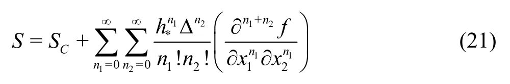
The use ofhrequires time step and grid spacing to decrease simultaneously, which is often ignored in previous CFD V&V. Simulation error is defined and evaluated by representing solutionSas a generalized Taylor series about a numerical benchmarkSC(estimated exact solution)

The second hypothesis is that numerical error and modeling error can be de-coupled and evaluated independently. With this hypothesis, the systematic grid and time-step refinement will be extended to also include the refinement of the filter width of the LES sub-grid scale models.

It should be noted there are disputes on how the numerical and modeling errors should be evaluated for LES. Some researchers[37,38](e.g. Eqs.(9) and (10)) varied the numerical and modeling parameters simultaneously whereas Oberkampf and Roy[21]suggested decoupling the numerical error and modeling error by fixing the filter width in LES sub-grid scale models when numerical errors are evaluated such that traditional systematic grid/time-step refinement for RANS V&V can be applied. Nonetheless, the default filterwidth for traditional/implicit LES is the local grid spacing. In such circumstances, simultaneous change of grid spacing and filter width may be inevitable. It is also ambiguous that what filter width should be fixed when there are at least three systematically refined grids. If the filter width is fixed at the smallest grid spacing on the fine grid, the LES solutions on the coarse and medium grids may be incorrect since filter widths on any grid cannot be smaller than its smallest grid spacing. It may be possible to fix the filter width at the coarse grid spacing but simulations on medium and fine grids will be a waste since some length scales are resolved in calculations but they are discarded by using a much larger filter width. It is even impossible to fix a filter width when the dynamic SGS model is used because the model requires the use of two filter widths in the simulation. It has been found by the author and his colleague that the filter width may also have significant influence on the simulation results and the sensitivity of the results to the filter width is different on different grids[43]. The general framework derived in this study will evaluate both approaches to determine their validity and possible correlations if any.

3.1 V&V methods of LES based on Hypothesis I

New systematic grid and model variation methods based on Hypothesis I are proposed, to quantitatively assess the numerical error, modeling error, and their coupling for LES.

3.1.1 H1-7 V&V method of LES-Seven equation estimator

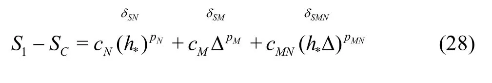
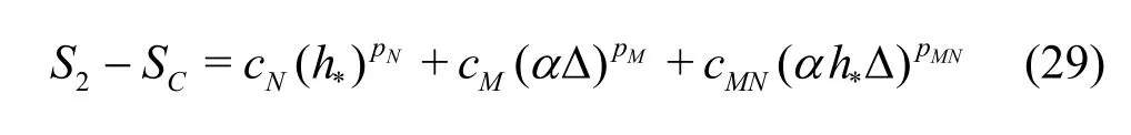
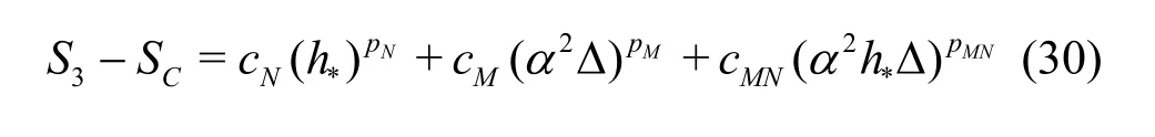
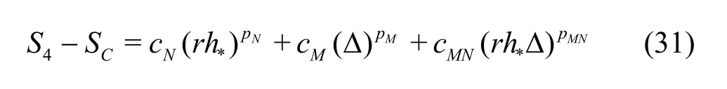
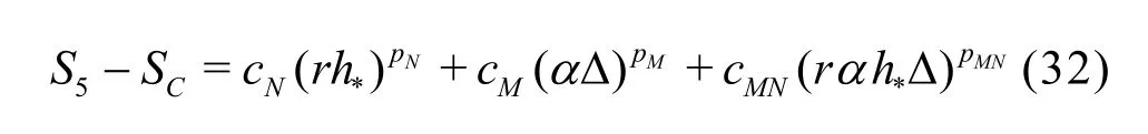
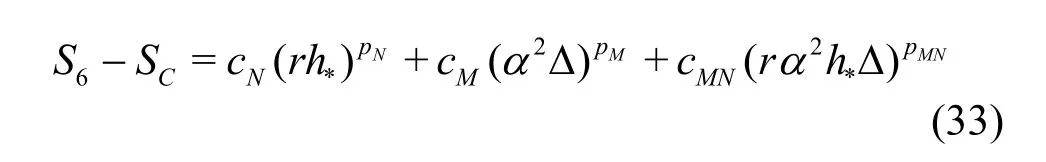
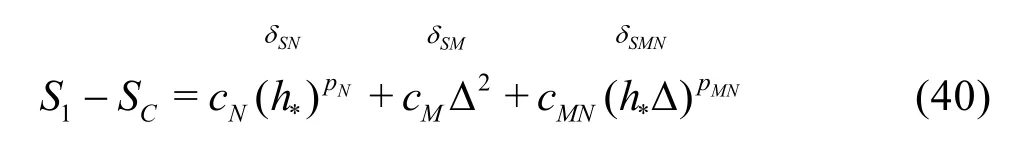
Compared to the existing method presented by Eqs.(8)-(13), the seven equation estimator has several significant improvements: (1) the effect of time step is evaluated simultaneously with the effect of grid refinement. As pointed out by Eca et al.[42-45], separate evaluation of the discretization uncertainty in gridand timeis incorrect. The grid spacing and time step should be refined simultaneously. This statement has been supported by Sathiah et al. who demonstrated that it is of utmost importance to apply successive mesh and time step refinement systematically in CFD for combustion models in hydrogen safety management[46]. Time step sizes can also significantly impact mean velocity field for turbulent flow in a mixing chamber[47]and maintain turbulence fluctuations in LES of a fully developed channel flow[48], (2)the observed order of accuracy for the numerical schemeN(Nplater) and for the SGS modelM(Mplater) are calculated rather than assumed. Additionally,a new termfor the coupling between numerical and modeling errors is added, (3) the grid spacing and filter width are separated such that the method is applicable to both implicitly and explicitly filtered LES, and (4) time-steptΔ, grid spacingh,and filter width Δ are varied for three, instead of two values. The new method extends the generalized Richardson Extrapolation for RANS to LES by representing the errors using a two-dimensional Taylor Series. Only the first leading terms are retained as higher order terms are much smaller. A constant grid and time step refinement ratioand a constant model variation factorare applied.As a result, seven equations for seven unknowns are needed as summarized below:

Fine grid with Δ

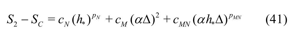
Fine grid withαΔ

Fine grid with2αΔ

Medium grid with Δ

Medium grid withαΔ

Medium grid with2αΔ

Coarse grid with Δ

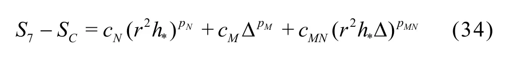
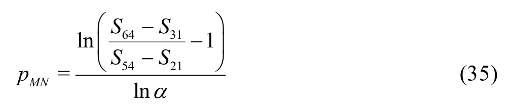
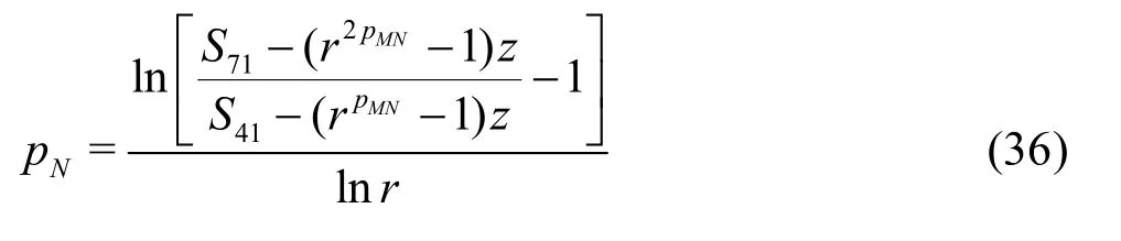
DenoteSij=Si-Sj, then seven unknowns can be solved

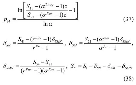
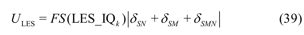
The uncertainty of the LES are estimated using Equation (39) has the advantage over Eq.(13) because it considers the circumstance that the numerical and modeling errors may have different signs and cancel each other out, which results in a small total error[35].Mathematically, there are two alternative ways to construct the seven equations, i.e., Eqs.(29) and (30) for the fine grid or Eqs.(32) and (33) for the medium grid may be replaced by solutions on the coarse grid with filter widths αΔ and2αΔ, respectively. Similarly,addition of solutions on the coarse grid with filter widths αΔ and2αΔ will allow users to construct three grid-triplet studies such that each has the same filter width, as suggested by Oberkampf and Roy[21]. The numerical errors and uncertainties can then be estimated using V&V for RANS. Accuracy and cost of the various estimators will be evaluated using an extensive database and statistical analysis discussed later.

3.1.2 H1-6 V&V method of LES−six equation estimator

The seven equation estimators are the most accurate but also the most expensive LES V&V method compared to existing approaches. In certain circumstances, implementation of the new method can be too expensive for some users due to the limitation of available computational resources. Thus, simplified versions of the general method need to be derived based on additional assumptions. IfNp is assumed to be equal tothp or the SGS modeling introduces a second-order dissipation term (i.e., pM=2), six-equation estimators can be derived. For example, if pM=2,the solution on the medium grid with filter width2αΔ can be discarded:

Fine grid with Δ

Fine grid with αΔ

Fine grid with2αΔ

Medium grid with Δ

Medium grid with αΔ

Coarse grid with Δ

It should be noted that there are several other ways to construct the six-equation estimator by dropping a different solution from the seven-equation estimator.The accuracy of different formulations needs to be evaluated.

3.1.3 H1-5 V&V Method of LES−Five equation estimator

If Np is assumed to be equal to thp and the SGS modeling introduces a second-order dissipation term(i.e., pM=2), a five-solution estimators can be derived. One possible formulation is to drop solutions on medium and fine grids with filter width2αΔ:

Fine grid with Δ

Fine grid with αΔ

Medium grid with Δ

Medium grid with αΔ

Coarse grid with ΔSimilarly to H1-6, there are several other ways to construct the five-equation estimator by dropping two different solutions from the seven-equation estimator.The accuracy of different formulations needs to be evaluated.

3.1.4 H1-1 V&V method of LES-Single-grid estimator

The LES index LES_IQkis used to construct the single-grid estimator: (1) If the total TKE is available(e.g., from DNS), LES_IQkis computed using Eq.(7).The total error is estimated using ktot- kresand uncertainty is computed using a modified version of Eq.(39)

(2) If the total TKE is unknown, it can be calculated using ktot= kres+keff_sgs. For implicitly or explicitly filtered LES that has the same filter width and grid spacing, the total, resolved, and modeled TKE can be calculated using the method described by the author[49,50]and Hedges et al.[51]. The errors and uncertainties can then be estimated using the same method discussed in (1). For explicitly filtered LES, where the filter width is different from the grid spacing, a single grid is insufficient to estimate errors and uncertainties and other methods must be used.

3.2 V&V methods of LES based on Hypothesis II

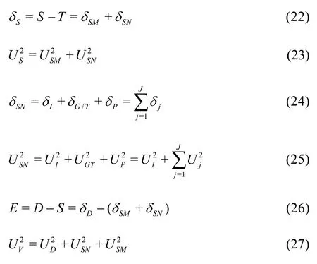
New systematic grid and model variation methods based on Hypothesis II are proposed, to quantitatively assess the numerical error and modeling error due to filter width for LES. The four improvements presented earlier for V&V methods using Hypothesis I are preserved. The difference is that the coupling term has been dropped and the numerical parameters (gridspacing and time-step) and filter width are independently evaluated by fixing one while systematically changing the other.

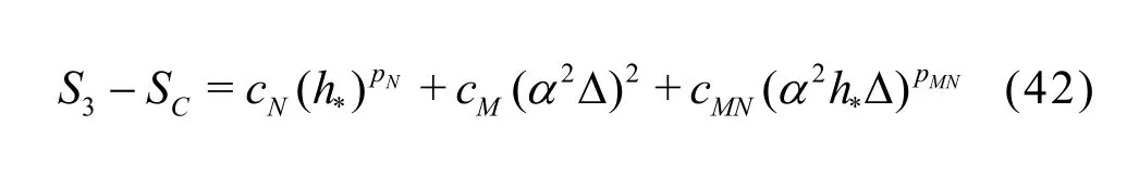
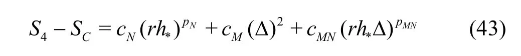
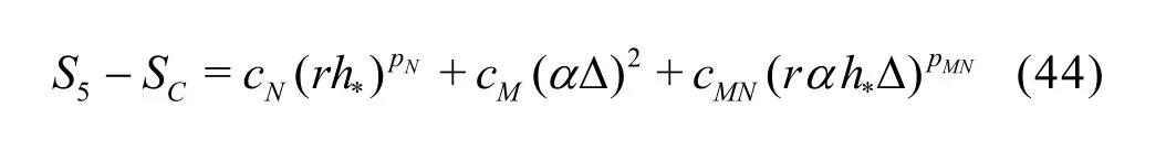
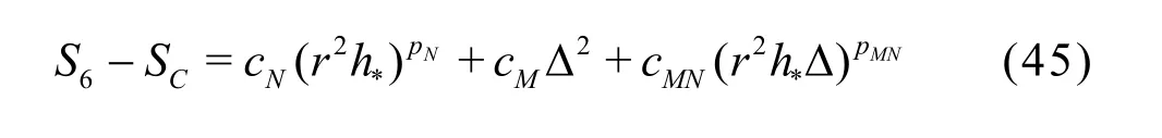
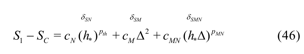
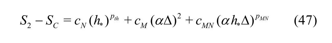
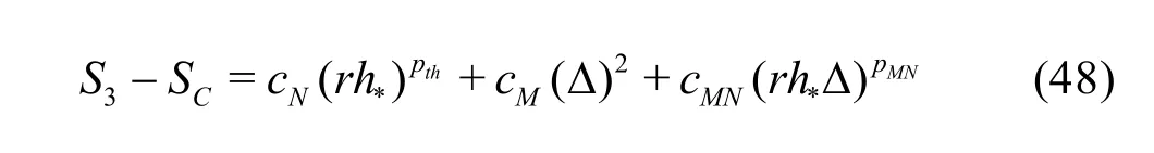
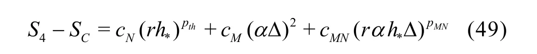
3.2.1 H2-5 V&V method of LES−Five equation estimator

A constant grid and time step refinement ratio rand a constant model variation factor αare applied. As a result, five equation estimator can be derived:

Fine grid with Δ

Fine grid with αΔ

Fine grid with2αΔ

Medium grid with Δ

Coarse grid with Δ

Denote Sij=Si-Sj, then five unknowns can be solved

The uncertainty of the LES are estimated using

Equation (59) has the advantage over Eq.(13) because it considers the circumstance that the numerical and modeling errors may have different signs and cancel each other out, which results in a small total error[35].Mathematically, there are two alternative ways to construct the five equations, i.e., Eqs.(53) and (54) for the fine grid may be replaced by the solutions on the coarse or medium grid with filter widths αΔ and2αΔ,respectively. Accuracy and cost of the three five-equation estimators needs to be evaluated using an extensive database and statistical analysis.

3.2.2 H2-3 V&V method of LES−Three equation estimator

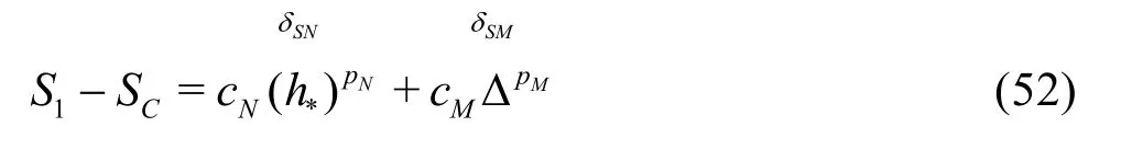
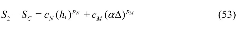
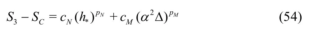
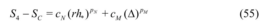
If the coupling term is dropped and assume pN=pthand pM=2[37], a three equation estimator can be derived. There are several other ways to construct the three equation estimator. For example, if Eqs.(52), (53)and (55) are used, the following formula can be used to compute the numerical and modeling error terms

The single-grid estimator is the same as that presented earlier based on Hypothesis I.

4. Large LES V&V database and statistical analysis

4.1 Extensive database

Previous LES V&V were derived and calibrated only for a small number of cases and flow conditions.This prohibits the use of these methods as general guidelines. The database approach as applied by Xing and Stern[24,25]to derive the factor of safety method for RANS will be extended to LES models to evaluate the new LES V&V methods. The new database will cover various geometries and flows at medium and high Reynolds numbers. Canonical flow cases include decaying homogeneous isotropic turbulence[39], transitional flat plate boundary layer[52], temporal mixing layer[53], plane turbulent jet[37], turbulent channel flow[54], turbulent flows in a driven cavity[55], external flow[56], and backward-facing step[57], etc.. Complex geometries will be selected in the field of ship hydrodynamics which the author is most familiar with, such as Wigley hull[58], KVLCC2 tanker[11,50], Athena with/without appendages[59,60], 5415[60], and submarine[10,61,62], etc.. Extensive experimental data and CFD simulations are available for those complex geometries because they have been used as well-known test cases for years in previous CFD Workshops[63,64].Other cases will be selected from public databases(ERCOFTAC Fluid Dynamics Database, NAS Data Set Archive, MADIC/NASA Code Certification,ASME Journal of Fluids Engineering, and NPARC Alliance Validation Archive). With the help of the senior faculty the author has been collaborating with over the past years, the author will build an expert network on CFD V&V such that many high fidelity LES results can be included in the database. Canonical flow cases will be focused for two reasons. First, reference solutions for complex geometries are difficult to obtain. Second, additional errors may be introduced when simulating flows for complex geometries, including insufficient iterative convergence[24]and grid aspect ratio, expansion ratio, and skewness[65]. Each case in the database will have at least one reference solution. For transitional or turbulent flows at moderateRe, the reference solution can be obtained using DNS. For highReturbulent flows, the manufactured solution will be used as the reference solution. The manufactured solution was mainly used in code verification. However, it can also be used to study the convergence characteristics of numerical solutions of partial differential equations such as the RANS models[66].

This method can also be applied for LES models.When manufactured solutions are difficult to develop,numerical benchmark will be used as the reference solution. Then at least seven LES as defined by Eqs.(28) to (34) will be performed for each case in the database. Additional LES will be performed when needed. Detailed information will be reported as electronic files using a standard format (geometry, flow conditions, grids, models, numerical methods, boundary and initial conditions, sampling time). The LES models to be evaluated include the Smagorinsky model[67], dynamic model[68,69], and other recently developed models available in commercial CFD software and CFD OpenFoam. Experimental data will also be included for each case, when available, for the purpose of validation. Through the expert network, the database will be expanded, continuously accessed, and dynamically interacted with and updated[70]. It will serve as a platform for collaboration between researchers in the world to study/evaluate CFD V&V.

4.2 Sample construction

The first step to construct a sample is to quantify the distance of an LES solution to DNS. The LES quality indices defined by Eq.(6) are difficult to use because of the insensitivity to grid refinement fors,many assumptions involved fors*, difficulty computing the Kolmogorov length scaleand difficulty estimatingdefined by Eq.(7) will be used to quantify the distance. Various samples of the database will be constructed in a manner similar to what the author did for the FS method for RANS[24]. The largest sample is for all the actual factor of safety itemswhereNis the sample size. For thethiV&V study of a sample,FSAiis defined as the ratio of the uncertainty estimateUSito the magnitude ofEi

The comparison errorEifor fine grid solution with smallest filter widthis

for an analytical benchmark such as the manufactured solution and

4.3 Determine FS (LES_IQk) and reliability using statistical analysis

Statistical analysis[24,25]will be performed based on the samples constructed to determinefor the seven-solution estimators. The error and uncertainty estimates are systematic, butEiand thereforeare treated as items drawn from the statistical and random parent population of possible systematic errors, which are similar to the systematic error in experimental measurements. Sinceare randomly distributed, the confidence interval for the mean reveals how close the mean value ofis to the true meanμof the parent population ofReliabilityRis defined as

The confidence of mean analysis is based on the methodology and procedures summarized in Ref.[71]. Ifis theitem of the sample with sizeN, the mean, the standard deviation, and the standard deviation of the mean of the sample are,, andrespectively. The true meanμof the parent population at the ninety-five percent confidence level is bounded by

4.4 Multi-objective optimal refinement and optimal regions for LES

Based on the extensive LES V&V database, a general guideline on the optimal combination of various numerical and modeling parameters will be derived to obtain the overall minimum errors for LES. Based on the LES results and the corresponding reference solution for each case, the overall simulation error based on the resolved TKE,, can be examined.Heredenotes a volume averaging. The error-landscape method based on weighted integrals of the energy spectrum[72-74]is modified as

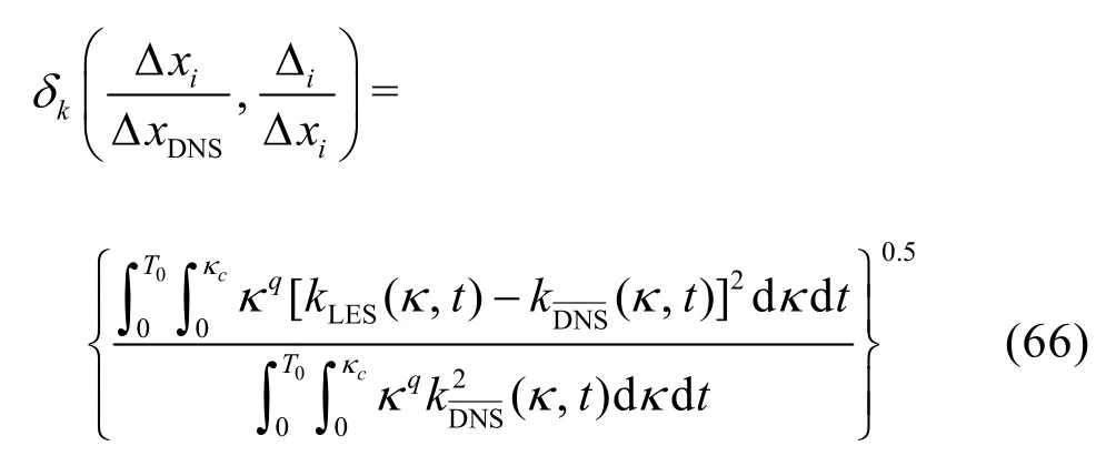
whereT0is the interrogation time window,κis the wave number, andκc= π/Δ is the grid cut-off frequency. Different values of the power exponentqof the wave number allows evaluations of error contributions in different wave number ranges[74]. Compared to the original definition of[72-74], the number of grid pointsNand the Smagorinsky coefficientCSare replaced by the grid spacing ratio and the subfilter resolution ratio[75,76], respectively. Since the grid and time-step are refined using the same ratior,is enforced and there is no need to include time step ratio in Eq.(66). These changes first improve the applicability of the formula: (1)conclusion of using it will be general as a result of using dimensionless parameters, (2) deletion ofCSallows the formula to be used for dynamic LES and other multiscale models, and (3)is an important index that indicates the distance to achieve “gridspacing independent” LES solutions[74,77]. Based on the error-landscape plot ofkδ, an “optimal refinement strategy” can be identified as the “valley” in this landscape[39].

Mixed discretization schemes are usually used for LES with the order of accuracy for the convective terms higher than or equal to that for the viscous terms.One may use fourth-order Runge-Kutta method for temporal discretization, fourth-order central schemefor convective terms, and second-order central difference for the viscous terms (4-4-2). Similarly, 2-4-2 or 2-2-2 may be used. To accommodate multiple errormeasures into the analysis, the “near-optimal” region[78]corresponding to the newkδdefined in Eq.(66)is used

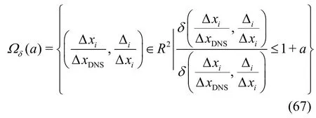
whereais a small positive number and arbitrarily specified to be 0.2 by Meyers et al.[72]. The extensive database will enable the author to provide guidelines on specifying “a.”

5. Extension of LES V&V

The developed V&V and optimization framework for LES models can be refined or modified to improve its applicability: (1) hybrid RANS/LES models use RANS and LES in different regions. The proposed framework needs to be modified to seamlessly connect the two models. One method is to use a blended function that is multiplied before the modeling and coupling terms such that it is zero and one in the RANS and LES regions, respectively, (2) for transitional flows, the new framework needs to be corrected in the laminar flow regimes because LES_IQ has no real meaning. One method is to introduce the laminar flow correction factor[36], and (3) special cases such as how to handle the negative values for the natural logarithm function as defined in Eq.(35). This is similar to the non-monotonic convergence cases for RANS/DES usually observed for industrial applications[50,59,60].The new framework proposed will help explain why these happen and provide guidelines on how to avoid them. When they are inevitable, the least square approach[29,45]will be extended for multiscale models.

The LES V&V framework can be extended for quantitative V&V for simulation of gas-liquid flows.DNS solutions for bubbly flows will be obtained from published literatures[79-81]and new simulations by the expert network.

V&V for bubbly flow is motivated by the fact that some bubbly flow models (without LES) have similar features to the LES SGS models, i.e., the model resolves different flow physics when the grid is refined. One example is Kubota’s cavitation model[81-85]that assumes a homogeneous mixture of liquid and spherical vapor bubbles. At scales below the grid size,cavitation regions are assumed to consist of locally homogeneous clusters of bubbles. The model expresses the nonlinear interaction between macroscopic vortex motion and microscopic bubble dynamics with interaction between bubbles

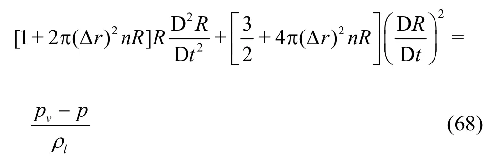
Herein,R,n, Δr,pv,pandlρare the bubble radius, bubble number density, bubble cluster radius(commonly chosen as local grid spacing), vapor pressure, fluid pressure, and liquid density, respectively.When Δr→0, the bubble/bubble interaction is neglected and the Rayleigh equation is recovered. The role of Δris similar to the filter width used in LES.Solution verification and optimization for the cavitating flows are similar to what was proposed earlier for LES (Eqs.(28)-(67)), but the filter width Δ is replaced by the bubble cluster radius Δr. This extension is applicable for laminar bubbly flow or turbulent bubbly flow with RANS models.

When LES is used for dispersed bubbly flow[86],the first step is to identify the scales at which the governing equations are to be solved: micro-, meso-, and macro-scales[87]. Noting that application of LES at a micro-scale is unrealistic for industrial-scale problems[88]and application of LES at a macro-scale leads to poor resolution of turbulence quantities[87], it is the authors’ suggestion that efforts should be focused on the meso-scale region, where the mesh size is comparable to bubble sizes. This extension aims to elucidate the optimum filter width for various bubble sizes to achieve the overall minimum simulation error and examine the numerical and modeling errors during grid and time step refinements. This will help resolve the conflict between the mesh requirement for multiphase modeling and the requirement by LES approaches[89].Solution verification and optimization are similar to what was proposed earlier for LES (Eqs.(28)-(67)),but Δris selected as Δr=constant × Δ and combined with the modeling error term such that the new modeling error terms becomes

6. Conclusion

The use of LES models in CFD has dramatically increased for academic research and industrial innovations. Nonetheless, existing V&V methods are mainly derived for RANS models and cannot be used for LES V&V and previous LES V&V has strong limitations.This study derived a general framework for LES V&V,which allows for quantitative estimations of numerical error, modeling error, their coupling, and the associated uncertainties on different numerical resolutions(e.g. grid, time-step, numerical schemes) and filter widths. Various LES V&V methods in this framework can meet different needs of users. Research outcomes using this general framework have the potential to significantly improve reliability, risk assessment, and decision making for a wide range of science and engineering applications. As such, this study has direct or indirect societal significance in protecting the environment, reducing cost of experiments, improving human health, and securing energy for the world. The reference solution and best solution using LES models in the database can be used as numerical benchmarks for future CFD simulations. The expert network on CFD V&V will also enhance the collaboration between worldwide researchers from different disciplines.

[1] JOHNSON F. T., TINOCO E. N. and YU N. J. Thirty years of development and application of CFD at boeing commercial airplanes, seattle[J]. Computers and Fluids, 2005, 34(10): 1115-1151.

[2] STERN F., YANG J. and WANG Z. et al. Computational ship hydrodynamics: Nowadays and way forward[J].International shipbuilding Progress, 2013, 60(1-4): 3-105.

[3] QUALLEN S., XING T. and CARRICA P. et al. CFD simulation of a floating offshore wind turbine system using a quasi-static crowfoot mooring-line model[J].Journal of Ocean and Wind Energy, 2014, 1(3): 143-152.

[4] QUALLEN S., XING T. and CARRICA P. et al.DISCUSSION: CFD Simulation of a floating offshore wind turbine system using a quasi-static crowfoot mooring-line model[J]. Journal of Ocean and Wind Energy, 2014, 1(3): 185-188.

[5] QUALLEN S., XING T. and CARRICA P. et al. CFD simulation of a floating offshore wind turbine system using a quasi-static crowfoot mooring-line model[C].23rd International Ocean and Polar Engineering Conference. Anchorage, USA, 2013.

[6] POPE S. B. Turbulent flows[M]. New York, USA:Cambridge university press, 2000.

[7] MAHESH K., CONSTANTINESCU G. and APTE S. et al. Large-eddy simulation of reacting turbulent flows in complex geometries[J]. ASME Journal of Applied Mechanics, 2006, 73(3): 374-381.

[8] YOU D., WANG M. and MOIN P. et al. Large-eddy simulation analysis of mechanisms for viscous losses in a turbomachinery tip-clearance flow[J]. Journal of Fluid Mechanics, 2007, 586: 177-204.

[9] YOU D., HAM F. and MOIN P. Discrete conservation principles in large-eddy simulation with application to separation control over an airfoil[J]. Physics of Fluids,2008, 20: 101515.

[10] FUREBY C. Large eddy simulation of ship hydrodynamics[C]. 27th Symposium on Naval Hydrodynamics.Seoul, Korea, 2008.

[11] XING T., CARRICA P. and STERN F. Large-scale RANS and DDES computations of KVLCC2 at drift angle 0 Degree[C]. A Workshop on CFD in Ship Hydrodynamics Gothenburg. Gothenburg, Sweden,2010.

[12] LI Y., PAIK K.-J. and XING T. et al. Dynamic overset CFD simulations of wind turbine aerodynamics[J]. Renewable Energy, 2012, 37(1): 285-298.

[13] WANG Z., SUH J. and YANG J. et al. Sharp interface LES of breaking waves by an interface piercing body in orthogonal curvilinear coordinates[C]. 50th AIAA Aerospace Sciences Meeting Including the New Horizons Forum and Aerospace Exposition. Nashville,Tennessee, USA, 2012.

[14] ASME. ASME guide on verification and validation in computational fluid dynamics and heat transfer[R]. Techical Report by ASME Performance Test Code Committee PTC-61, ANSI Standard V&V-20, 2008.

[15] STERN F., WILSON R. V. and COLEMAN H. W. et al.Comprehensive approach to verification and validation of CFD simulations-Part 1: Methodology and procedures[J]. Journal of Fluids Engineering, 2001, 123(4):793-802.

[16] COLEMAN H., STERN F. Uncertainties and CFD code validation[J]. Journal of Fluids Engineering, 1997,119(4): 795-803.

[17] ROACHE P. J. Verification and validation in computational science and engineering[M]. Socorro, New Mexico, USA: Hermosa Publishers, 1998.

[18] ROACHE P. J. Fundamentals of verification and validation[M]. Socorro, New Mexico, USA: Hermosa Publishers, 2009.

[19] CELIK I. B., GHIA U. and ROACHE P. J. et al. Procedure for estimation and reporting of uncertainty due to discretization in CFD applications[J]. Journal of Fluids Engineering, 2008, 130(7): 078001.

[20] COSNER R. R., OBERKAMPF W. L. and RUMSEY C.L. et al. AIAA committee on standards for computational fluid dynamics: Status and plans[C]. 44th AIAA Aerospace Sciences Meeting and Exhibit. Reno,Nevada, USA, 2006, AIAA 2006-889.

[21] OBERKAMPF W. L., ROY C. J. Verification and validation in scientific computing[M]. New York, USA:Cambridge University Press, 2010.

[22] STERN F., WILSON R. and SHAO J. Quantitative V&V of CFD simulations and certification of CFD codes[J]. International Journal for Numerical Methods in Fluids, 2006, 50(11): 1335-1355.

[23] WILSON R., SHAO J. and STERN F. Discussion: Criticisms of the “correction factor” verification method[J].Journal of Fluids Engineering, 2004, 126(4): 704-706.

[24] XING T., STERN F. Factors of safety for Richardson extrapolation[J]. Journal of Fluids Engineering, 2010,132(6): 061403.

[25] XING T., STERN F. Closure to “Discussion of “Factors of safety for Richardson extrapolation” (2011, Journal of Fluids Engineering, 133: 115501), Journal of Fluids Engineering, 2011, 133(11): 115502.

[26] CELIK I., HU G. Single grid error estimation using error transport equation[J]. Journal of Fluids Engineering, 2004, 126(5): 778-790.

[27] EÇA L., HOEKSTRA M. An evaluation of verification procedures for CFD applications[C]. 24th Symposium on Naval Hydrodynamics. Fukuoka, Japan, 2002.

[28] EÇA L., HOEKSTRA M. and BEJA PEDRO J. F. et al.On the characterization of grid density in grid refinement studies for discretization error estimation[J]. Interna-tional Journal for Numerical Methods in Fluids,2013, 72(1): 119-134.

[29] EÇA L., HOEKSTRA M. Discretization uncertainty estimation based on a least squares version of the grid convergence index[C]. Proceedings of the Second Workshop on CFD Uncertainty Analysis. Lisbon,Portugal, 2006.

[30] PHILLIPS T. S., ROY C. J. Richardson extrapolationbased discretization uncertainty estimation for computational fluid dynamics[J]. Journal of Fluids Engineering, 2014, 136(12): 121401.

[31] VIOLA I., BOT P. and RIOTTE M. On the uncertainty of CFD in sail aerodynamics[J]. International Journal for Numerical Methods in Fluids, 2013, 72(11): 1146-1164.

[32] OBERKAMPF W. L., TRUCANO T. G. Validation methodology in computational fluid dynamics[C]. AIAA 2000-2549, Fluids 2000 Conference and Exhibit.Denver, USA, 2000.

[33] GEURTS B. J., FRӧHLICH J. A framework for predicting accuracy limitations in large-eddy simulation[J].Physics of Fluids, 2002, 14(6): L41-L42.

[34] GEURTS B. J. Balancing errors in LES, direct and large-eddy simulation III[M]. Dordrecht, The Netherlands: Springer, 1999, 1-12.

[35] CELIK I. B., CEHRELI Z. N. and YAVUZ I. Index of resolution quality for large eddy simulations[J]. Journal of Fluids Engineering, 2005, 127(5): 949-958.

[36] CELIK I., KLEIN M. and JANICKA J. Assessment measures for engineering LES applications[J]. Journal of Fluids Engineering, 2009, 131(3): 031102.

[37] KLEIN M. An attempt to assess the quality of large eddy simulations in the context of implicit filtering[J].Flow, Turbulence and Combustion, 2005, 75(1-4):131-147.

[38] FREITAG M., KLEIN M. An improved method to assess the quality of large eddy simulations in the context of implicit filtering[J]. Journal of Turbulence, 2006,7(40): 1-11.

[39] MEYERS J., GEURTS B. J. and BAELMANS M. Database analysis of errors in large-eddy simulation[J].Physics of Fluids, 2003, 15(9): 2740-2755.

[40] TRAVIN A., SHUR M. and STRELETS M. et al. Detached-eddy simulations past a circular cylinder[J].Flow, Turbulence and Combustion, 2000, 63(1): 293-313.

[41] SAGAUT P., DECK S. Large eddy simulation for aerodynamics: Status and perspectives[J]. Philosophical Transactions of the Royal Society A: Mathematical,Physical and Engineering Sciences, 2009, 367(1899):2849-2860.

[42] EÇA L., HOEKSTRA M. Code verification of unsteady flow solvers with the method of the manufactured solutions[C]. 17th International Offshore and Polar Engineering Conference. Lisbon, Portugal, 2007.

[43] XING T., SHAO J. and STERN F. BKW-RS-DES of unsteady vortical flow for KVLCC2 at large drift angles[C]. The 9th international conference on Numerical Ship Hydrodynamics. Ann Arbor, Michigan, USA,2007.

[44] EÇA L. Private communication to T. Xing[R]. 2014.

[45] EÇA L., VAZ G. and HOEKSTRA M. Code verification, solution verification and validation in RANS solvers[C]. 29th International Conference on Ocean,Offshore and Arctic Engineering. Shanghai, China,2010.

[46] SATHIAH P., KOMEN E. and ROEKAERTS D. The role of CFD combustion modeling in hydrogen safety management-Part I: Validation based on small scale experiments[J]. Nuclear Engineering and Design, 2012, 248: 93-107.

[47] STERNEL D. C., SCHÄFER M. and GAUß F. et al. Influence of numerical parameters for large eddy simulations of complex flow fields[J]. European Conference on Compuational Fluid Dynamics, ECCOMAS CFD 2006. Egmond aan Zee, The Netherlands, 2006.

[48] PARK T. Effects of time-integration method in a largeeddy simulation using the PISO algorithm: Part I-Flow field[J]. Numerical Heat Transfer, Part A: Applica- tions, 2006, 50(3): 229-245.

[49] XING T., KANDASAMY M. and STERN F. Unsteady free-surface wave-induced separation: analysis of turbulent structures using detached eddy simulation and single-phase level set[J]. Journal of Turbulence, 2007, 8(44): 1-35.

[50] XING T., BHUSHAN S. and STERN F. Vortical and turbulent structures for KVLCC2 at Drift Angle 0, 12,and 30 degrees[J]. Ocean Engineering, 2012, 55: 23- 43.

[51] HEDGES L. S., TRAVIN A. K. and SPALART P. R.Detached-eddy simulations over a simplified landing gear[J]. Journal of Fluids Engineering, 2002, 124(2): 413-423.

[52] NOLAN K. P., ZAKI T. A. Conditional sampling of transitional boundary layers in pressure gradients[J]. Journal of Fluid Mechanics, 2013, 728: 306-339.

[53] VREMAN B., GEURTS B. and KUERTEN H. Comparison of numerical schemes in large-eddy simulation of the temporal mixing layer[J]. International Journal for Numerical Methods in Fluids, 1996, 22(4): 297- 297.

[54] MOSER R. D., KIM J. and MANSOUR N. N. Direct numerical simulation of turbulent channel flow up toRe=590[J]. Physics of Fluids, 1999, 11(4): 943-945.

[55] VERSTAPPEN R., WISSINK J. G. and CAZEMIER W.et al. Direct numerical simulations of turbulent flow in a driven cavity[J]. Future Generation Computer Syste- ms, 1994, 10(2-3): 345-350.

[56] WISSINk J. G., RODI W. Numerical study of the near wake of a circular cylinder[J]. International Journal of Heat and Fluid Flow, 2008, 29(4): 1060-1070.

[57] HUNG L., MOIN P. and KIM J. Direct numerical simulation of turbulent flow over a backward-facing step[J].Journal of Fluid Mechanics, 1997, 330: 349-374.

[58] PINTO-HEREDERO A., XING T. and STERN F.URANS and DES analysis for a Wigley hull at extreme drift angles[J]. Journal of Marine Science and Tech- nology, 2010, 15(4): 295-315.

[59] XING T., CARRICA P. and STERN F. Computational towing tank procedures for single run curves of resistance and propulsion[J]. Journal of Fluids Engineering, 2008, 130(10): 101102.

[60] BHUSHAN S., XING T. and CARRICA P. et al.Model- and full-scale URANS simulations of athena aesistance, powering, seakeeping, and 5415 maneuvering[J]. Journal of Ship Research, 2009, 53(4): 179- 198.

[61] FUREBY C. ILES and LES of complex engineering turbulent flows[J]. Journal of Fluids Engineering, 2007, 129(12): 1514-1523.

[62] FUREBY C. Towards the use of large eddy simulation in engineering[J]. Progress in Aerospace Sciences,2008, 44(6): 381-396.

[63] LARSSON L., STERN F. and BERTRAM V. Benchmarking of computational fluid dynamics for ship flows:The Gothenburg 2000 workshop[J]. Journal of Ship Research, 2003, 47(1): 63-81.

[64] LARSSON L., STERN F. and VISONNEAU M. CFD in ship hydrodynamics-results of the Gothenburg 2010 workship[C]. MARINE 2011-IV International Conference on Computational Methods in Marine Engineering. Lisbon, Portugal, 2011.

[65] ISMAIL F., CARRICA P. M. and XING T. et al. Evaluation of linear and nonlinear convection schemes on multidimensional non-orthogonal grids with applications to KVLCC2 tanker[J]. International Journal for Numerical Methods in Fluids, 2010, 64: 850-886.

[66] EÇA L., VAZ G. and HOEKSTRA M. Assessing convergence properties of RANS solvers with manufactured solutions[C]. European Congress on Computational Methods in Applied Sciences and Engineering(ECCOMAS 2012). Vienna, Austria, 2012.

[67] SMAGORINSKY J. General circulation experiments with the primitive equations: I. The basic experiment[J].Monthly Weather Review, 1963, 91(3): 99-164.

[68] GERMANO M., PIOMELLI U. and MOIN P. et al. A dynamic subgrid-scale eddy viscosity model[J]. Physics of Fluids A: Fluid Dynamics, 1991, 3(7): 1760-1765.

[69] LILLY D. K. Proposed modification of the Germano subgrid-scale closure method[J]. Physics of Fluids A:Fluid Dynamics, 1992, 4(3): 633-633.

[70] RIZZI A., VOS J. Toward establishing credibility in computational fluid dynamics simulations[J]. AIAA Journal, 1998, 36(5): 668-675.

[71] KREYSZIG E. Advanced engineering mathematics[M]. 7th Edition, New York, USA: Wiley, 2007.

[72] MEYERS J., GEURTS B. and SAGAUT P. A computational error-assessment of central finite-volume discretizations in large-eddy simulation using a Smagorinsky model[J]. Journal of Computational Physics, 2007,227(1): 156-173.

[73] MEYERS J. Error-landscape assessment of largeeddy simulations: A review of the methodology[M].New York, USA: Springer, 65-77.

[74] GEURTS B. J. Analysis of errors occurring in large eddy simulation[J]. Philosophical Transactions of the Royal Society A: Mathematical, Physical and Engineering Sciences, 2009, 367(1899): 2873-2883.

[75] GHOSAL S. An analysis of numerical errors in largeeddy simulations of turbulence[J]. Journal of Computational Physics, 1996, 125(1): 187-206.

[76] KRAVCHENKO A., MOIN P. On the effect of numerical errors in large eddy simulations of turbulent flows[J]. Journal of Computational Physics, 1997,131(2): 310-322.

[77] RADHAKRISHNAN S., BELLAN J. Explicit filtering to obtain grid-spacing-independent and discretizationorder-independent large-eddy simulation of two-phase volumetrically dilute flow with evaporation[J]. Journal of Fluid Mechanics, 2013, 719: 230-267.

[78] MEYERS J., SAGAUT P. and GEURTS B. J. Optimal model parameters for multi-objective large-eddy simulations[J]. Physics of Fluids, 2006, 18(9): 095103.

[79] NIERHAUS T., VANDEN ABEELE D. and DECONINCK H. Direct numerical simulation of bubbly flow in the turbulent boundary layer of a horizontal parallel plate electrochemical reactor[J]. International Journal of Heat and Fluid Flow, 2007, 28(4): 542-551.

[80] BOLOTNOV I. A., JANSEN K. E. and DREW D. A. et al. Detached direct numerical simulations of turbulent two-phase bubbly channel flow[J]. International Journal of Multiphase Flow, 2011, 37(6): 647-659.

[81] XING T. Numerical modeling and simulation of laminar and transitional submerged cavitating jets[D]. Doctoral Thesis, West Lafayette, USA: Purdue University,2002.

[82] KUBOTA A., KATO H. and YAMAGUCHI H. A new modelling of cavitating flows: A numerical study of unsteady cavitation on a hydrofoil section[J]. Journal of Fluid Mechanics, 1992, 240: 59-96.

[83] SHI Su-guo, WANG Guo-yu. A modified kubota cavitation model for computations of cryogenic cavitating flows[J]. Chinese Journal of Theoretical and Applied Mechanics, 2012, 44(2): 269-277.

[84] XING T., FRANKEL S. H. Effect of cavitation on vortex dynamics in a submerged laminar jet[J]. AIAA Journal, 2002, 40(11): 2266-2276.

[85] XING T., LI Z. and FRANKEL S. H. Numerical simulation of vortex cavitation in a three-dimensional submerged transitional jet[J]. Journal of Fluids Engineering, 2005, 127(4): 714-725.

[86] WANG G., OSTOJA-STARZEWSKI M. Large eddy simulation of a sheet/cloud cavitation on a NACA0015 hydrofoil[J]. Applied Mathematical Modelling, 2007,31(3): 417-447.

[87] DHOTRE M. T., DEEN N. G. and NICENO B. et al.Large eddy simulation for dispersed bubbly flows: A review[J]. International Journal of Chemical Engineering, 2013.

[88] BESTION D. Applicability of two-phase CFD to nuclear reactor thermalhydraulics and elaboration of best practice guidelines[J]. Nuclear Engineering and Design, 2012, 253: 311-321.

[89] NIČENO B., DHOTRE M. T. and DEEN N G. Oneequation sub-grid scale (SGS) modelling for Euler-Euler large eddy simulation (EELES) of dispersed bubbly flow[J]. Chemical Engineering Science, 2008,63(15): 3923-3931.