Rank regression: an alternative regression approach for data with outliers

Tian CHEN, Wan TANG, Ying LU, Xin TU*

•Biostatistics in psychiatry (23)•

Rank regression: an alternative regression approach for data with outliers

Tian CHEN1, Wan TANG1, Ying LU2, Xin TU1*

normal distribution, non-normal distribution, linear regression, semi-parametric regression models, rank regression, sexual health

1. Introduction

Regression is widely used in mental health research and related services research to model relationships involving health and service utilization outcomes and clinical and socio-demographic factors. Regression models measure changes in the dependent variable in response to changes in a set of independent variables of interest. Linear regression focuses on continuous dependent variables, while other regression models such as logistic and log-linear regression consider noncontinuous dependent variables such as binary and count outcomes. The dependent variable is often called the response, while the independent variables are frequently referred to as the explanatory variables,predictors, or covariates.

Linear regression is arguably the most popular regression model in practice, because of the ubiquity of continuous outcomes and because it is relatively easy to understand the modeled relationship and interpret the model estimates. Fitting such models is convenient because all major software packages (R,SAS, SPSS and STATA) provide both the model estimates and the diagnostics of the model fit. However, the wide popularity and routine use of the linear regression also creates some problems. Many researchers apply the model without first checking assumptions about the normal distribution of the data underlying the validity of model estimates. The classic normal-based linear regression imposes strong constraints on data, and its estimates are also quite sensitive to departures from assumed mathematical models. Without careful checking of the model assumptions, estimates generated by linear regression models may be difficult to interpret and conclusions drawn from such estimates may be misleading.

2. Different approaches to deal with non-normal study data in regression analyses

Classic linear regression assumes a normally distributed response,yi, and models the mean of this response variable as a function of a set of independent variables,xi= (xi1 , xi2 ...., xip)Tas follows∶

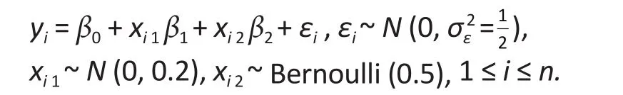
whereβ= (β1, β2, ..., βp)Tis the vector of parameters,nis the sample size,εidenotes the error term,N(µ,σ2)denotes a normal distribution with meanµand varianceσ2, andεi～N(0,σ2) means thatεifollows a normal distribution with mean 0 and varianceσ2. The wellshaped bell curve of the normal distribution is often at odds with the distribution of data arising in real studies,because of its symmetric shape and extremely thin tails(exponential decay). Over the years, various methods have been developed to improve the limitations of the classic linear model. All the different methods can be grouped into 3 major categories.

One approach is to use mathematical distributions that more closely resemble the data distribution in the study.[1]For example, by positing a t-distribution for the errorεi, the resulting linear model can accommodate data distributions with thicker tails. This is possible because the t-distribution has an additional degree of freedom parameter to control the thickness of the tail.However, like the normal distribution, the t-distribution is also symmetric. To model skewed data distributions,a popular approach is to use the chi-square distribution.Although this parametric alternative broadens the scope of data distributions that can be accommodated, it is still quite limited because mathematical distributions always have more regular shapes than those arising in practice.

A second popular alternative is to use semiparametric or distribution-free models.[2]Under this approach, no mathematical model is assumed for the data distribution (the non-parametric part) and the relationship betweenyiandxiis represented by the mean ofyiafter adjustment forxi(parametric component). The latter parametric component is implied by the specification of the classic linear regression in (1)and is given by∶

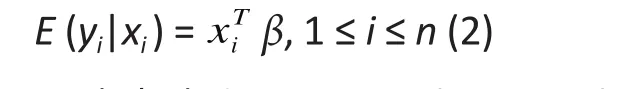
whereE(yi|xi) denotes mathematical expectation. For those unfamiliar with mathematical expectation, the above expression simply means that the population-level average of the responseyiis a linear function ofxi. This linear relationship is also implicit in the normal-based linear regression in (1). Thus, the semi-parametric linear model in (2) only requires a linear relationship between the response and the set of explanatory variables,thereby offering valid inference for a wide class of data distributions.

Although significantly improving the utility of linear regression, the semi-parametric model still has limited applications. A major problem is that like the classic model it continues to model the mean of the response.Like the sample mean of a variable, model estimates from this approach can be quite biased when there are extremely large or small values, or outliers, in the response.

Various approaches have been developed to address this important issue of outliers. A common approach in psychosocial research is to trim outliers using ad-hoc rules. For example, limiting the values of all observations to 3 times the interquartile range when estimating the mean of an outcome (i.e., a ‘trimmed’mean).[3]However, these ad-hoc methods induce artifacts because of their dependence on the specific rules used, and the use of different rules can result in different outcomes.

Another approach to limiting the influence of outliers is to employ rank tests. The Mann-Whitney-Wilcoxon rank sum test is widely used to compare two groups in such situations. Within the setting of regression analysis, rank regression is a popular approach for dealing with outliers.[4,5]Like the Mann-Whitney-Wilcoxon rank sum test, rank regression does not use the observed responsesyidirectly, but,rather, uses information about the ranking of these observations, thereby yielding estimates that are much less sensitive to outliers.

3. Simulation studies to compare different approaches

The data were simulated from a study with one binary variable and one continuous covariate. To show differences across the different methods, we selected a large sample size (n=500) to reduce the effect of sampling variability on model estimates. We performed simulation of data and fitted the different models to the data generated using the R software. All simulations were performed with a Monte Carlo sample size M=1000 and a type I errorα=0.05.

We simulatedyifrom the following linear model∶

We then simulated 50 (or 10% of the sample size) values from a uniformU(500, 1000000), ordered them as∶

and added the valuesu(1)from the uniform to the 50 largest values ofyi, i.e.,

to form a set of outlying observations, i.e.,

To assess the robustness of the different methods,we replacedy(451)＜y(452)＜ ...＜ y(500)in the original sample with the valuesz(451)＜z(452)＜ ...＜ z(500), and fit the models to the resulting observations∶

Table 1 shows the estimates ofβ1andβ2, the corresponding standard errors, and type I error rates from fitting the three methods to data simulated from the normal-distributed errorN(0, 1/2) based on 1000 Monte Carlo simulations both with and without included outliers. (The interceptβ0is estimated by the rank regression and so this estimate is missing in the table.) In the table, values in the column titled‘mean’ are the averaged estimates of each parameter over 1000 Monte Caro replications; the ‘asymptotic standard error’ is the model-based standard error; the‘empirical standard error’ is the standard errors of the 1000 estimates of each parameter; and the ‘type I error’is the percent of times the null hypothesis - that the estimated parameter is equal to the true parameter -is rejected. For example, the empirical type I error rates forβ1in the data set without outliers is the percent oftimes of rejecting the nullH0∶β1=1.

If a model performs well, (a) the averaged value of estimates of each parameter (in the ‘mean’ column)should be close to the true value of the respective parameter; (b) the magnitude of the asymptotic standard error should be close to that of the empirical standard error; and (c) the empirical type I error rate should be close to the nominal value 0.05. As shown in Table 1, in the absence of outliers, all three methods performed well, with the averaged estimates all nearly identical to the true value 1, the asymptotic standard errors all close to their empirical counterparts, and the type I error rate all close to the nominal levelα=0.05.Further, all three methods yielded near identical standard errors, indicating that there is practically no loss of power by using the two robust alternatives instead of the classic linear model for the simulated normal data.

However, results are very different in the presence of outliers. As shown in the Table 1, both the classic and semi-parametric models yielded extremely large estimates that are un-interpretable, impossibly large standard errors, and type I errors close to 1. In contrast,the rank regression model for bothβ1andβ2generated estimates close to the true value 1, reasonable asymptotic and empirical standard errors that were equal to each other, and type I errors that, though elevated, were close to the nominal 0.05 level.

Table 2 shows the results of a similar simulation when the data were simulated from t-distributed error, ,instead of from normal-distributed error. In the absence of outliers the mean estimate and type 1 error of the two parameters were acceptable for all three models;however, the empirical standard error was much larger than the asymptotic standard error for the classical and semi-parametric models while these two types of standard error were similar in magnitude in the rank regression model. In the presence of outliers, as was the case in the normal-error simulation, the estimates generated by the classic and semi-parametric models were un-interpretable while those generated by the rank regression model were acceptable. Thus, for data with t-distribution error the rank regression model preforms better than the classic linear and the semiparametric models both in the absence and in the presence of outliers.

4. A real-life example

To illustrate the three approaches to dealing with outliers, we use results from a recent randomizedcontrolled study[6]to evaluate the efficacy of a sexual risk-reduction intervention program targeting teenage girls in low-income urban settings who are at elevated risk for HIV, sexually transmitted infections, and unintended pregnancies. The study recruited sexuallyactive urban adolescent girls aged 15 to 19 and randomized them to a sexual risk reduction intervention or to a structurally-equivalent health promotion control group. Assessments and behavioral data were collected at baseline, 3, 6 and 12 months post-baseline.The primary interest of the study was to compare the frequency of unprotected vaginal sex between the two treatment conditions. A difficult problem with the study data was the extremely large values reported by some subjects for their sexual activities. For example, five subjects reported over 100 episodes of unprotected vaginal sex over the past 3 months at the 6 month follow-up. If linear regression is applied directly to this outcome, estimates will be severely biased and become un-interpretable. Alternative models need to be considered when analyzing the data.

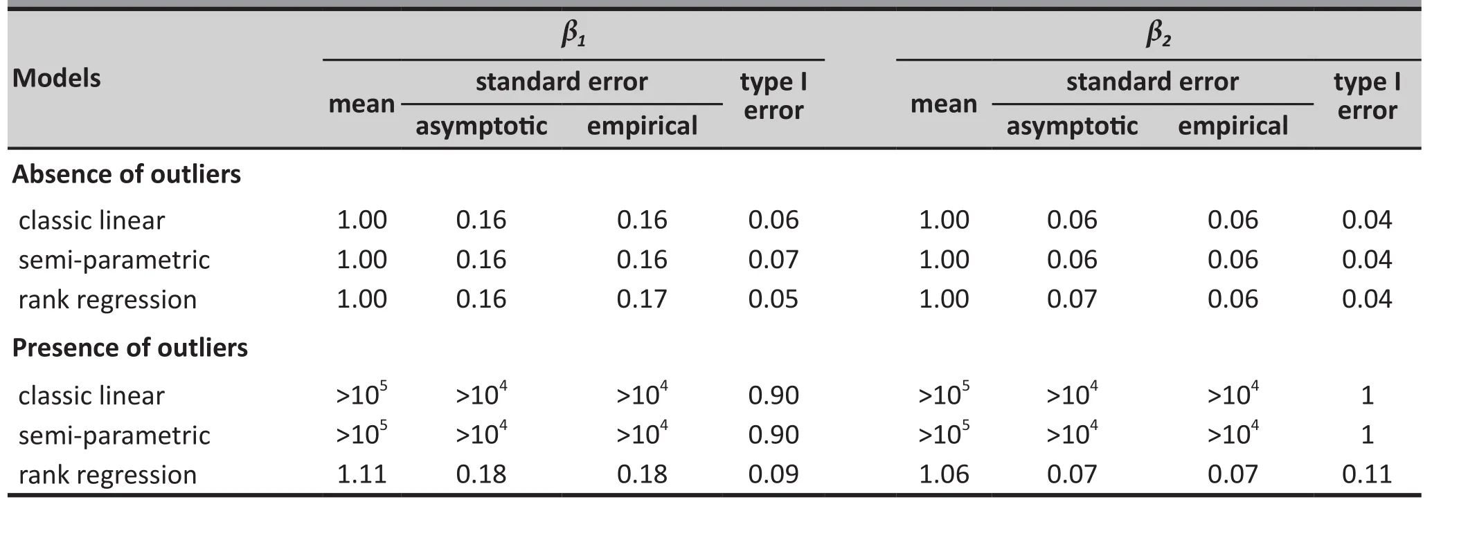
Table 1. Estimates (mean), asymptotic and empirical standard errors, and empirical type I error rates from fitting the classic linear, semi-parametric, and rank regression models to data simulated from normal-distributed errors

The linear regression for the different methods is specified as follows∶

whereyiis the number of episodes of unprotected vaginal sex,xi1is the binary indicator for the treatment condition (1 for the intervention and 0 for the control group), andεiis the model error. The model errorεifollows the normal distribution for the classic linear regression, while the distribution is unspecified for the semi-parametric and rank regression methods.

To highlight the differences in the models we removed zero observations (i.e., individuals who reported no episodes of unprotected sex in the prior three months) and fit all three models (classic linear,semi-parametric, and rank regression) to the remaining data. In addition, we also recomputed the estimates for the classic linear model and the semi-parametric model after trimming the observed responses to decrease the influence of outliers. We trimmed the observed responses of number of episodes of unprotected vaginal sex in the prior three months at 3 times the interquartile range; the 25%, 50% and 75% quartiles were 2, 4, and 10 episodes, respectively, so the interquartile range was 8 (10 - 2) and any observations below -20 (4 - 3*8)or above +28 (4 + 3*8) were considered outliers. There were no observations below -20 so no lower-level trimming was necessary, but all observations above 28 were trimmed to 28.

Table 3 shows the resulting estimates ofβ1for the treatment condition in the linear model (3) and the corresponding asymptotic standard errors and p-values using the different models. As was the case in the simulation study with outliers, the huge values for the estimates and standard errors using the classic linear and semi-parametric models clearly show that the estimates are profoundly affected by the outliers and,thus, are un-interpretable. In comparison, the classic and semi-parametric methods yielded more reasonable estimates when applied to the trimmed observations.However, results using the trimmed data were still quite different from those generated from the rank regression model; the estimates from the two models that used trimmed data were more than 50% higher than that using the rank regression method and the standard errors were more than double that from the rank regression analysis. Results from the simulation study suggest that rank regression is quite robust against outliers and, unlike models that use trimmed data,are not vulnerable to change when different trimming criteria are employed.

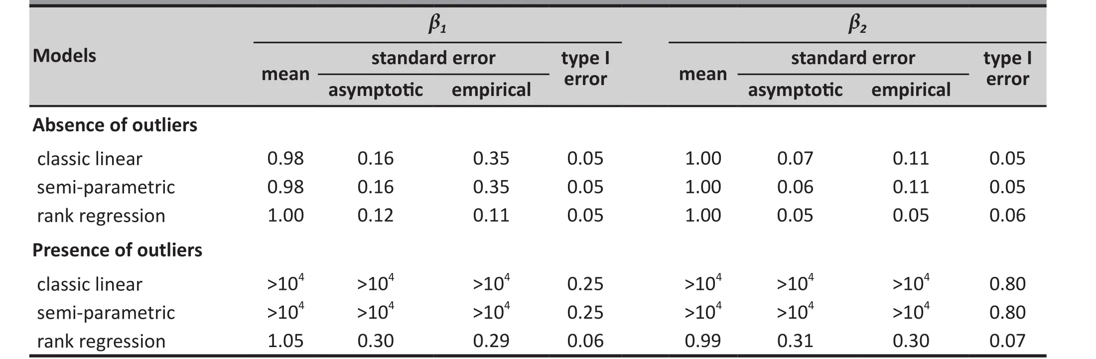
Table 2. Estimates (mean), asymptotic and empirical standard errors, and empirical type I error rates from fitting the classic linear, semi-parametric, and rank regression models to data simulated from t-distributed errors

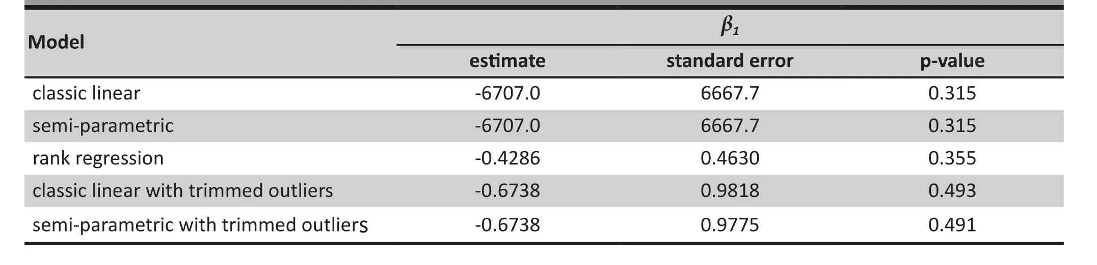
Table 3. Estimates, standard errors, and p-values from fitting the classic linear, semi-parametric,rank regression, classic linear with trimmed outliers, and semi-parametric with trimmed outliers models to the risk-reduction intervention study

5. Sotfware for alternative linear regression models

Most major software such as R and SAS has the capability of fitting the semi-parametric linear regression model. In R, there are several packages available for fitting the generalized estimating equations (GEE).Although GEE is an extension of the semi-parametric method for longitudinal data, we may still use these packages for fitting the semi-parametric model to crosssectional data by introducing an ‘ID’ variable that has unique values for each of the observations. For example,if the GEE package is installed, then one may apply the following codes to fit the semi-parametric linear regression model∶

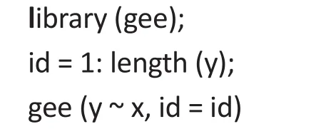
where y is the outcome and x is the covariate matrix.

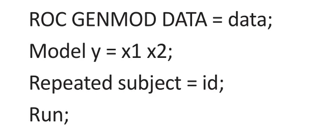
Similarly, SAS also offers ‘Procedures’ for fitting the GEE which can be utilized to provide estimates for semiparametric linear regression models. For example, by adding an ID variable to the SAS data set, we may apply the Procedure GENMOD to fit the semi-parametric model∶

At the time of writing, SAS does not have the capability to fit the rank regression. For our simulated and real study examples, packages in R were used to fit this robust alternative model. To perform this regression model, first download the R functions from the website∶http∶//www.stat.wmich.edu/mckean/HMC/Rcode/AppendixB/ww.r. Then, we use the following command in R to obtain estimates from fitting the rank regression∶

where y is the outcome and x is the covariate matrix.

Note that while SAS is a commercial software package, R is free to download, install, and run. In addition, software for newer statistical methods are generally first available in R. However, unlike SAS, R has no designated technical support so users generally rely on peer-support, web postings, and books for resolving issues concerning applications of specific packages and general data management problems.

6. Discussion

Classic linear regression has a number of weaknesses,limiting its applications to real study data. We discussed two robust alternatives, the semi-parametric model and the rank regression model. Although the former yields more valid estimates than the classic linear model, it breaks down when there are extremely large (or small)observations in the response (i.e., the dependent variable). In the presence of such outliers, the rank regression model provides much more robust estimates.Unlike ad-hoc methods such as trimming outliers based on 3 x interquartile range, rank regression generates the same estimates regardless of the actual values of the response as long as the rankings of the observations remain the same. This formal approach not only removes any subjective element in the estimates, but it also makes it easier to compare results of different analyses based on the same study data and to compare results between different studies. Further, the rank regression model is also capable of addressing outliers in the independent variables, although this tutorial only discussed outliers in the response variable.

Currently, rank regression is only available in some selected software packages such as R - we included sample R codes for fitting this robust regression model in this report to facilitate its use by readers. As this approach becomes more popular, it is likely that other major software giants such as SAS will have similar offerings.

Unlike the classic and semi-parametric linear regression models, rank regression is only available for fitting cross-sectional data. This is, in part, due to the complexity of computing estimates and asymptotic standard errors. However, as longitudinal studies become the norm rather than the exception in modern clinical research, it will become increasingly important to develop software that can extend this robust model to longitudinal research data and, thus, help investigators more effectively deal with imperfections in real study data.

Conflict of interest

The authors report no conflict of interest related to this manuscript.

Funding

The preparation of this manuscript was supported in part by DA027521 and GM108337 from the National Institutes of Health.

1. Kowalski J, Tu XM, Day RS, Mendoza-Blanco JR. On the rate of convergence of the ECME algorithm for multiple regression models with t-distributed errors.Biometrika. 1997; 84∶269-281. doi∶ http∶//dx.doi.org/10.1093/biomet/84.2.269

2. Tang W, He H,Tu XM.Applied Categorical and Count Data Analysis. Boca Raton, Florida, USA∶ Chapman & Hall/CRC Press. 2012

3. Schroder EB, Liao DP, Chambless LE, Prineas RJ, Evans GW,Heiss G. Hypertension, blood pressure, and heart rate variability∶ the Atherosclerosis Risk in Communities (ARIC)study.Hypertension.2003; 42(6)∶ 1106-1111. doi∶ http∶//dx.doi.org/10.1161/01.HYP.0000100444.71069.73

4. Jaeckel LA. Estimating regression coefficients by minimizing the dispersion of the residuals.Ann Math Statist. 1972;43(5)∶ 1449-1458

5. Jureckova J. Nonparametric estimate of regression coefficients.Ann Math Statist.1971; 42(4)∶ 1328-1338

6. Morrison-Beedy D, Jones S, Xia Y, Tu XM, Crean H, Carey M. Reducing sexual risk behavior in adolescent girls∶results from a randomized controlled trial.J Adolesc Health.2013; 52∶ 314-321. doi∶ http∶//dx.doi.org/10.1016/j.jadohealth.2012.07.005

∶ 2014-10-08; accepted∶ 2014-10-10)

Ms. Tian Chen is a fifth-year PhD student in the Department of Biostatistics and Computational Biology, School of Medicine and Dentistry, University of Rochester. Her PhD thesis focuses on semiparametric and rank-based statistical models, and variable selection methods for regression models for both cross-sectional and longitudinal data. She has applied these statistical methods in the analysis of mental health and related research.

等级回归：离群数据的另一种回归方法

Tian CHEN, Wan TANG, Ying LU, Xin TU

正态分布，非正态分布，线性回归，半参数回归模型，等级回归，性健康

Summary:Linear regression models are widely used in mental health and related health services research.However, the classic linear regression analysis assumes that the data are normally distributed, an assumption that is not met by the data obtained in many studies. One method of dealing with this problem is to use semi-parametric models, which do not require that the data be normally distributed. But semi-parametric models are quite sensitive to outlying observations, so the generated estimates are unreliable when study data includes outliers. In this situation, some researchers trim the extreme values prior to conducting the analysis, but the ad-hoc rules used for data trimming are based on subjective criteria so different methods of adjustment can yield different results. Rank regression provides a more objective approach to dealing with non-normal data that includes outliers. This paper uses simulated and real data to illustrate this useful regression approach for dealing with outliers and compares it to the results generated using classical regression models and semi-parametric regression models.

[Shanghai Arch Psychiatry. 2014; 26(5)∶ 310-316. doi∶ http∶//dx.doi.org/10.11919/j.issn.1002-0829.214148]

1Department of Biostatistics and Computational Biology, University of Rochester, NY, USA

2Department of Biostatistics, Stanford University, Stanford, CA, USA

*correspondence∶ xin_tu@urmc.rochester.edu

A full-text Chinese translation of this article will be available at www.shanghaiarchivesofpsychiatry.org on November 25, 2014.

概述: 线性回归模型被广泛应用于精神卫生和卫生服务相关研究。然而，经典线性回归分析是假设该数据为正态分布的，但是很多研究所获得的数据并不符合这种假设。解决该问题的方法之一是采用不要求数据为正态分布的半参数模型。但是，半参数模型对离散数据相当敏感，因此在处理包含离散值的数据时产生的估计值是不可靠的。在这种情况下，一些研究者在删减这些极端值后再进行分析，但是，删减数据的事先法则（ad-hoc rules）是基于主观标准的，所以不同的调整方法就会产生不同的结果。等级回归为处理包括离散值的非正态分布数据提供了更为客观的方法。本文采用虚拟和实际数据来阐述这个非常有用的处理离散值的回归方法，并与采用经典回归模型和半参数回归模型所得出的结果进行比较。

本文全文中文版从2014年11月25日起在www.shanghaiarchivesofpsychaitry.org可供免费阅览下载