Modeling household car ownership using ordered logistic regression model

Deng Yiling Guo Xiucheng

(School of Transportation, Southeast University, Nanjing 210096, China)



Modeling household car ownership using ordered logistic regression model

Deng Yiling Guo Xiucheng

(School of Transportation, Southeast University, Nanjing 210096, China)

Considering both the discrete and ordered nature of the household car ownership, an ordered logistic regression model to predict household car ownership is established by using the data of Nanjing Household Travel Survey in the year 2012. The model results show that some household characteristics such as the number of driver licenses, household income and home location are significant. Yet, the intersection density indicating the street patterns of home location, and the dummy near the subway and the bus stop density indicating the transit accessibility of home location are insignificant. The model estimation obtains a goodγ2(the goodness of fit of the model) and the model validation also shows a good performance in prediction. The marginal effects of all the significant explanatory variables are calculated to quantify the odds change in the household car ownership following a one-unit change in the explanatory variables.

household car ownership; ordered logistic regression model; marginal effect; household characteristics; neighborhood characteristics

The number of cars available to a household has a major impact on the travel behavior of the household members. Car ownership models estimate the number of cars owned by households based on the characteristics of the households themselves, the characteristics of the neighborhoods where they are located and the accessibilities of those neighborhoods via various transportation modes. While the estimation of car ownership is not one of the four classic steps of traditional travel demand model—the four-step model, the availability of cars to households affects trip generation, trip distribution and mode choice. To produce credible forecasts of travel demand, it is desirable not only to have accurate estimates of the households and employment for transportation analysis zones, but also to have accurate estimates of the number of cars available to those households. As a result, some travel demand models have incorporated the components of the household car ownership model.

There are three commonly used approaches in car ownership models: aggregate approaches, disaggregate approaches and dynamic approaches. Aggregate approaches estimate the total number of households for each vehicle ownership category at the city or region level in future years. Time-series extrapolations using aggregate data reflecting the economic development level at city or regional level are the most common methods. According to the general rule observed in industrialized countries, sigmoid-shaped curves are usually adopted to model the growth in car ownership[1]. Three other types of curves that have been used to simulate the growth in car ownership in some research are: the power function curves, the logistic curves and the Gompertz curves[2]. Disaggregate approaches model the probability of each household owning zero, one, two or more cars. These approaches were characterized by the use of the discrete choice model and maximum likelihood estimation[2]. These approaches appear to date from the work of Lerman and Ben-Akiva[3]in the US and Daly and Zachary[4]in the UK. Disaggregate approaches rely on household level information and can reveal individual behavior explicitly, which greatly improves the quality of the models. The probabilities output from the disaggregate approaches can also be applied to aggregate forecasting.

Both the first two types of approaches are static, which estimate the total number of cars in the city or transportation analysis zones (aggregate approaches) or the probability of a household owning a particular number of cars (disaggregate approaches) at a specific time. The dynamic approaches model the car transaction processes of each household in a time period rather than only model the final outcomes. Dynamic approaches, also called microsimulation, are considered as the most advanced method in modeling car ownership[5-6]. These approaches were reviewed by de Jong and Kitamura[7], who pointed out the necessity in some cases for undertaking a more complicated modelling of transactions, i.e. household interventions in the car market, rather than holdings. The effects captured by dynamic approaches operate over a 3-5 year period for households and over perhaps a 10-year period for the market as a whole, as older car types are scrapped and replaced by newer types. Additional data in addition to household travel survey data is required to estimate such models. These models are usually used incorporated with some advanced activity-based models or integrated land use and transportation models.

The aggregate approaches are used in most operational four-step models implemented in Chinese cities. In these models, the car ownerships are estimated at the city level, assuming that car ownerships follow some trends such as the sigmoid curve over the forecast years. Then, the total car ownerships are assigned to each transportation analysis zone according to some zonal demographic, social-economic or land use attributes. Although these aggregate models are easy to use, they cannot reveal the behavior mechanisms by which households make the decision to acquire a car because many household and personal attributes available in household travel surveys cannot be included in these models. The dynamic approaches are the most behavior realistic, but also the most complicated. In the context of the practices in Chinese cities, the disaggregate approaches are the most appropriate methods at this time. They are more behavior realistic than the aggregate approaches, and can be integrated into the four-step model seamlessly without any additional data.

1 Methodology

The discrete choice model family is most capable of modelling the household car ownership—a categorical variable. If the household car ownership is modeled following an unordered response mechanism, the multinomial logit model will be used as most previous studies have been carried out in this way. The multinomial logit model assumes each car ownership level has a random utility. The household will select the ownership level with the highest utility, consistent with global utility maximization.

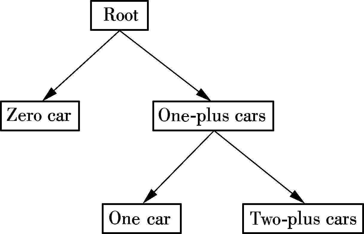
If the household car ownership is modeled following an ordered response mechanism, the ordered logistic regression model will be the most appropriate technique. Other than the multinomial logit model, in which utility is alternative specific, the alternatives in the ordered logistic regression model share the same formation and parameters of the utility function. The model uses thresholds in order to distinguish the different ownership levels on the underlying propensity. Fig.1 shows its choice structure. It can be understood as a series of binary choice decisions. At the first choice level, the household makes the choice to own zero or one-plus cars. Then, the household which passes the threshold of owning one-plus cars makes the decision to own only one car or two-plus cars.

Fig.1 The choice structure of the ordered logistic regression model

Ordered logistic regression models take the form

Y*=X·β+ε

(1)

whereY*is the unobserved dependent variable;Xis the vector of independent variables;βis the vector of regression coefficients to be estimated; andεis a random disturbance term. The observed ordinal variableYis a function ofY*, which has various category thresholds. For example,

(2)

The ordered logistic regression model uses the observations onYto determine the parameter vectorβand the threshold valuesμ1andμ2, so as to be able to subsequently estimateY*and predictYfor specific configurations ofX. Ifεis assumed to be independently Gumbel distributed across observations, then an ordered logistic regression model results in the selection probabilities,

(3)

whereΦ(·) is the cumulative distribution function of logistic distribution.

2 Data

The data used for our car ownership model is from the Nanjing Household Travel Survey 2012. It is an official survey conducted by the Nanjing Institute of City & Transport Planning Co., Ltd. Nanjing is the capital of Jiangsu Province, China. It covers an area of 4723 km2and had a population of 8.16 million in 2012[8]. Typical of many other Chinese cities, Nanjing is experiencing dramatic and rapid urbanization, economic growth, and motorization. Between 1980 and 2010, Nanjing’s gross domestic product (GDP) grew by more than 10% per year (in real terms), and its population increased from 4.7 to 8.0 million[8]. The Nanjing Household Travel Survey interviewed 6000 individuals in 2 005 households in the year 2012. The database includes household attributes such as car ownership and household income, personal characteristics for each household member such as gender, age and occupation, and a one-day travel diary for each participant.

As a household level model, the initial estimation data where all the households were analyzed in the household travel survey, contained 2005 records. The initial estimation data was then filtered to remove the records which had unreported household income. Finally, 1 900 records remained in the final estimation data.

2.1 Dependent variable

Tab.1 shows the frequency of household car ownership. Zero car households and one car households account for 96.8% of total household samples. Only 0.3% households own three cars. Considering the small proportion of the three-car alternative, it was reasonable to use a single alternative to represent the ownership of two or more cars.

Tab．1 Observed frequency of household car ownership

2.2 Explanatory variables

A number of tests were undertaken to determine the most competitive explanatory variables. Finally, two variable categories were defined in our model.

2.2.1 The demographic and socioeconomics characteristics of the household

The household structure in particular, the number of household members, is an important determinant of the household car ownership level. It is expected that the larger households have higher mobility needs and need to own more cars in order to improve their mobility. However, different types of household members have different mobility needs. Working adults are expected to have the greatest, followed by students. Preschool children and retirees may have the least mobility needs. The working adults are the potential drivers in the household. The students, preschool children and retirees may need to be given a ride by them to satisfy their needs for mobility. Taking the consideration of household responsibility of car ownership into account is the main reason to operate the car ownership model at household level. The age of householder is another indicator of the household structure. It was dummy coded because it may have a nonlinear effect on the household car ownership level. Four dummy variables were included in the model to represent five categories of the age of householders (20-30, 30-40, 40-50, 50-60, 60 or more).

The number of driver licenses directly relates to the potential maximum household car ownership. Household income is another important explanatory variable. It is expected that the richer the households, the greater the potential to own more cars. The household incomes were recorded using seven different bins (0-10000, 10000-20000, 20000-50000, 50000-100000, 100000-150000, 150000-200000, 200000 or more) in the household travel survey data, and were converted into a continuous variable by using the mid-point for each income band. 250 000 was selected to represent the top income bin considering the overall income level of Nanjing.

2.2.2 The urban transportation characteristics of the neighborhood

The urban form characteristics of the neighborhood where the household lives include the location, the street network pattern and transit service. The Manhattan distance to Xinjiekou, the central business district(CBD) of Nanjing, was used to represent the home location.

作为小学教师，应当走出传统教学模式的束缚，做到以人为本，重视学生的主体地位，真正结合学生的认知能力、心理特点和年龄特性，合理开发和利用教育资源，通过信息化、多媒体的教学手段，来让学生真正参与其中，发挥他们的主观能动性，通过多样化、个性化的信息学习体验，来帮助学生更深入地学习理论知识。

The intersection density is the most direct variable employed to characterize the street network pattern. It was measured using the number of intersections, excluding cul-de-sacs, per square kilometer in the neighborhood. The intersection density is also an indicator of the connectivity of the street network, which plays a significant role in the encouragement of non-motorized trips. The greater the intersection density, the more route choices for the pedestrian and cyclist, the more likely a person will walk and cycle.

The public transit and the car drive are substitution modes in the urban transportation market. Accessing higher quality public transportation is expected to reduce the number of cars owned by a household. The transit accessibility was measured using bus stop density (the number of bus stops per square kilometer in the neighborhood) and dummy near the subway (whether the home is located within the 800 m walkshed area of the subway station).

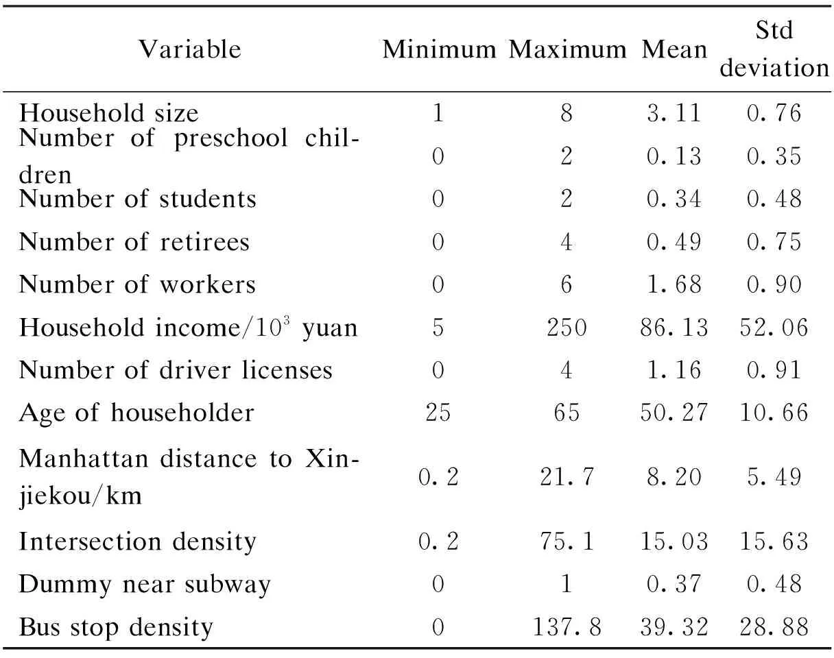
All the above mentioned explanatory variables are summarized in Tab.2, including their descriptive statistics.

Tab．2 Descriptive statistics of explanatory variables

Note: As the household income and age of householder are categorical variables, the mid-points of all categories are used to compute the statistics.

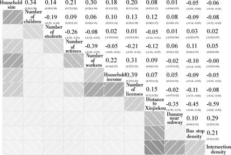
The correlations of all the explanatory variables need to be tested to make sure that all the variables are not highly correlated. It was done by generating Pearson correlation coefficients for all pairwise combinations as shown in Fig.2. The diagonal cells are the names of variables. The cells in the lower triangular show the shade plots of each variable pairs. The larger the absolute value of the correlation coefficient, the darker the shade. The corresponding cells in the upper triangular show the correlation coefficients and their 95% confidence intervals. The larger the absolute value of the correlation coefficient, the higher the two variables’ correlation. As the chart shows, the household size and the Manhattan distance to Xinjiekou have wide correlations with all other variables, however, they are not too high to be removed in advance. The household size is positively correlated with the number of preschool children (0.34), the number of workers (0.30), the number of retirees (0.21) and the number of driver licenses (0.20). The Manhattan distance to Xinjiekou is negatively correlated with the intersection density (-0.59), transit density (-0.49) and dummy variable of near subway (-0.35).

Fig.2 The correlation chart of explanatory variables

3 Model Analysis

3.1 Model estimation

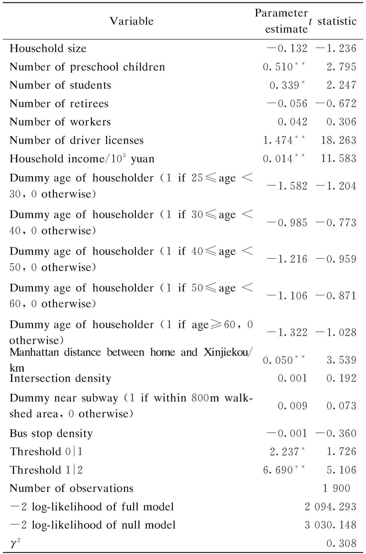
The maximum likelihood estimation is used to estimate the model. The parameter specification of the car ownership model is detailed in Tab.3. The model shows a reasonable goodness of fit withγ2of 0.308. All the parameters which are significant have the predictable signs.

The probability of owning one or more cars increases with the number of driver licenses. The effects are all plausible. The parameter for the household income is positive and very significant. Higher car ownership levels will be expected in high income households. However, the age of the householder effects are all insignificant.

Additionally, it was found that car ownership increases strongly as distance from Xinjiekou increases. This variable may relate to the characteristics of different areas, e.g. areas further from the CBD may be generally better suited for car ownership; certainly there is an increase in trip length, and a decline in public transport use, when residences are further from the CBD.

Other three variables that were found to be insignificant were intersection density, bus stop density and dummy near subway. Accordingly, the increase in the number of cars owned by a household increases the car availability and thus improves accessibility for all members of the household, including those who do not have licenses. The improvement is less in areas which are more walkable or have a higher transit service level. However, this theory fails to consider the self-selection effect, that is, high income households are more likely to live in the areas with abundant amenities and public services (also including transit services).

Tab．3 The parameters and tstatistic of the car ownership model

Note:*indicates that the parameter is significant at 5% percent;**indicates that the parameter is significant at 1% percent.

3.2 Model validation

The model was validated by applying it to the estimation data. The prediction success table is shown in Tab.4, which indicates similar results to the estimation set. 73.7% of the household car ownerships was correctly predicted. The model appears to be more accurate for the zero- and one-car levels, but less so for the two-plus-car level. The total number of the zero- and one-car levels is closely matched. The small amount of observation data for the two-plus-car level makes it difficult to estimate and predict the two-plus-car choice.

Tab．4 Confusion matrix of the prediction and observation

3.3 Marginal effects

To assess the overall effect of the explanatory variables on the three car ownership levels, marginal effects are computed for each observation and then averaged across all observations. The marginal effects show the effect that a one-unit change in explanatory variable has on each of the car ownership categories (zero, one, and two-plus). Tab.5 presents the marginal effects with respect to the average number of cars in a household. The results show that the number of driver licenses is the variable with the highest impact on car ownership with a marginal effect of 4.37. Regarding driver licenses, we would say that for a one-unit increase in driver licenses, e.g., the odds of a 2 driver license household “own two-plus cars” vs. “own one car” and “own zero car” combined is 4.37 times that of a 1 driver license household, given that all of the other variables in the model are held constant. Likewise, the odds of a 2 driver license household “own two-plus cars” and “own one car” combined vs. “own zero car” is 4.37 times that of a 1 driver license household, given that all of the other variables in the model are held constant. For household income, the interpretation is that when the household income moves one unit upward, i.e., increasing by 1 000 yuan, the odds of moving from “own two-plus cars” to “own one car” or “own zero car” (or from the lower and middle categories to the high category) are multiplied by 1.01. It is also important to notice that if a household is located 1 km far away from Xinjiekou, it has 1.05 times odds to own more cars.

Tab．5 Marginal effects of the explanatory variables

4 Conclusion

Revealing the mechanism of acquiring a car and modeling the car ownership precisely are important for urban transportation planning and policy making. In this paper, the ordered logistic regression model is adopted to model the household car ownership in Nanjing. The model shows fairly good results with theγ2of 0.307 and 73.7% of the household car ownerships being correctly predicted when we validate the model using the estimation data. All the significant variables have the predictable signs. The marginal effects of all the significant explanatory variables are calculated, which quantify the odds change in the household car ownership following a one-unit change in the explanatory variables. The final results indicate that the ordered logistic regression model is an attractive alternative to traditional aggregate approaches or multinomial discrete-outcome modeling methods such as the multinomial logit model used in car ownership modeling.

The car ownership model can also be extended to incorporate other variables in further research, for example, the land use terms such as the density, diversity and design of the home and other accessibility terms such as the logsum from the commute destination choice model. Such terms make the car ownership models sensitive to the changes of land use planning and transportation policy. However, adding these terms introduces additional complexity to the implementation.

[1]Ögüt K S. S-curve models to determine the car ownership in Turkey [J].ARI,theBulletinoftheIstanbulTechnicalUniversity, 2004, 54(2): 65-69.

[2]Jong G D, Fox J, Daly A, et al. Comparison of car ownership models [J].TransportReviews, 2004, 24(4): 379-408.

[3]Lerman S R, Ben-Akiva M. Disaggregate behavior model of automobile ownership [J].TransportationResearchRecord, 1976(569): 34-55.

[4]Daly A, Zachary S. The effect of free public transport on the journey to work [R]. Berkshire, England: Transport and Road Research Laboratory, 1977.

[5]Mohammadian A, Miller E J. Dynamic modeling of household automobile transactions [J].TransportationResearchRecord:JournaloftheTransportationResearchBoard, 2003, 1831: 98-105.

[6]Roorda M J, Mohammadian A, Miller E J. Toronto area car ownership study: a retrospective interview and its applications [J].TransportationResearchRecord:JournaloftheTransportationResearchBoard, 2000, 1719: 69-76.

[7]De Jong G C, Kitamura R. A review of household dynamic vehicle ownership models: holdings models versus transactions models [J].Transportation, 2009, 36(6):733-743.

[8]National Bureau of Statistics of the People’s Republic of China.Chinacitystatisticalyearbook[M].Beijing, China: China Statistics Press, 2013.(in Chinese)

基于序次logistic回归模型的家庭小汽车拥有量建模

邓一凌 过秀成

(东南大学交通学院, 南京 210096)

基于南京市2012年居民出行调查数据,建立了能同时考虑家庭小汽车拥有量的离散属性和序次属性的序次logistic回归模型，对家庭小汽车拥有量进行预测.模型结果表明：一些家庭属性比如家庭驾照持有数量、收入水平和居住位置对家庭小汽车拥有量有显著的影响，而表征家庭所在社区街道模式的变量(交叉口密度)和表征家庭所在社区公共交通可达性的变量(是否在地铁站步行范围内及公共交通站点密度)对家庭小汽车拥有量的影响并不显著.模型总体拟合度γ2和模型检验结果均表明该模型总体表现良好.最后计算了所有显著的解释变量的边际效应，即解释变量1个单位变化能够引起的家庭小汽车拥有量概率的变化.

家庭小汽车拥有;序次logistic回归模型;边际效应;家庭属性;社区属性

U491

Received 2014-03-10．

Biographies：Deng Yiling (1987—), male, graduate; Guo Xiucheng (corresponding author), male, doctor, professor, seuguo@seu.edu.cn.

：Deng Yiling, Guo Xiucheng．Modeling household car ownership using ordered logistic regression model[J]．Journal of Southeast University (English Edition),2014,30(4):500-505．

10.3969/j.issn.1003-7985.2014.04.017

10.3969/j.issn.1003-7985.2014.04.017