Experimental Model and Analytic Solution for Real-time Observation of Vehicle’s Additional Steer Angle

ZHANG Xiaolong ,LI Liang, *,PAN DengCAO Chengmaoand SONG Jian

1 School of Engineering,Anhui Agricultural University,Hefei 230036,China

2 State Key Laboratory of Automotive Safety and Energy,Tsinghua University,Beijing 100084,China

1 Introduction*

Active yaw moment control(AYC)is the main module of vehicle electronic stability control system(ESC).It resorts to the accurate adjusting of wheel force to control the whole vehicle’s motion.But of great importance,the vehicle's steering characteristics should be identified dynamically[1].Once a large steering input is added,the vertical load of inside wheels will be transferred to the outside wheels,and at the same time the road will produce a large sideslip force induced by the centrifugal force of the whole vehicle.Just the large sideslip force resulting in a distortion of suspension guide rod system,a small angle turning of wheel plane around the main pin is generated,i.e.,compliance steer.Meantime,the roll motion of vehicle body installed over the suspension will produce roll steer angle caused by the centrifugal force of the whole vehicle.The generation reason of roll steer also includes the equivalent movement effect of suspension distortion caused by the uneven road.Generally,it is difficult to make a clear distinction between compliance steer and roll steer while carrying out road way test,so they are comprehensively referred as additional steer angle in this paper.As a part of wheel’s sideslip angle,the additional steer angle can increase the trend of under-steering or over-steering,consequently has a significant influence on vehicle dynamic steering characteristics[2].

The current research on ESC mainly focused on the vehicle state observation[3–4],the control algorithm[5–6]and its test methods[7].However,few of them investigated the testing and modeling of additional steer angle.In general,only vehicle lateral acceleration was taken into consideration for observation of additional steer angle[8–9].The K&C properties of different vehicles may vary largely.As a result,the characteristics of additional steer angle also vary to different extent.The observation accuracy resorting to this method cannot meet the requirements of vehicle real time stability control,especially under the extreme driving conditions.

This paper will firstly analyze the influencing factors on the additional steer angle based on the simulation experiments,then establishes an observation model of additional steer angle using support vector machine(SVM)method,whose input vector elements are limited as the ESC configuration sensor information.The established observation model should take both the real-time and the accuracy of evaluation into consideration,so as to meet the AYC control requirements under complex driving conditions.

2 Vehicle Model and Verification

The multi-body dynamics simulation model of a passenger vehicle was built with ADAMS/Car platform,which includes front &rear suspension system,steering system,brake system,front &rear wheel models and chassis systems.In the model,the ISO coordinate system was used,and its origin point was located at the intersection of vehicle left &right symmetry plane and front wheel rotation axis when the vehicle was driven straight.As shown in Fig.1,X-axis and Y-axis point to the rear and right side of the vehicle respectively,and both axes are parallel with the ground when vehicle is still,while Z-axis points upwards,i.e.,perpendicular to the ground.The main parameters of the model are shown in Table 1.

Fig.1.Vehicle multi-body dynamic model

Table 1.Main parameters of vehicle model

2.1 Extraction of steering angle of front wheel

The test vehicle employs the independent front suspension with double wishbone,and the rack &pinion steering system.Thus the steering system has the characteristics of simple structure,flexible layout and reliable transmission.The left-front suspension structure is shown in Fig.2(a).

During the simulation test,the steering angle of front wheel cannot be achieved directly.It requires to establish a request command and to extract it through model solver[10].An extraction example of the operation of left-front wheel turning to the right is shown in Fig.2(b).Because the front wheel is rotated around the outer half axle 6,they can be regarded as a whole in other directions.Two sequential points p1and p2along the outer half axle are taken from the outside of vehicle body to the inner side,which are marked(x1,y1,z1)and(x2,y2,z2),respectively in the coordinate system of vehicle body.Therefore,the left-front wheel steer angle can be expressed as

Fig.2.Structure of left-front suspension and extraction method of steering angle of front wheel

Similarly,the right-front wheel steer angle can be extracted by establishing the same request command based on the right-front suspension.

2.2 Establishment of road model

In order to simulate compliance steer motion induced by uneven road,a three-dimensional model of the sinusoidal road(road_3d_sine_example.rdf)was built.Fig.3 shows a side view of the 3D road.

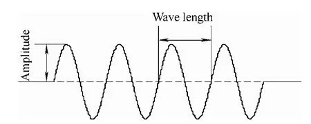
Fig.3.Diagram of sinusoidal road wave

2.3 Establishment of simulation driver file

The simulation driver files were obtained by modifying the templates of typical driver conditions in ADAMS software.In this paper,the driver files of steady static circular tests with fixed hand-wheel angle were created to verify the accuracy of vehicle simulation model established above,and some other driver files for tests,such as step steering,constant velocity,acceleration and deceleration,and so on,were also created to analyze the influencing factors of additional steer angle.Besides,the driver files of slalom and FMVSS 126 tests were created to build the SVM model and to test its generalization ability.All the file types were *.xml or *.dcf.

2.4 Verification of vehicle simulation model

The accuracy of vehicle simulation model was verified by comparing the simulation test data with its roadway test data under the same driving conditions.As shown in Fig.4,the steady static circular test was adopted,in which the steering angle of hand wheel was fixed at a constant value and the vehicle was driven in uniform acceleration until the sideslip of any axle happened.The extracted parameters used to make comparison include velocity,lateral acceleration,yaw rate,steering radius and roll angle of vehicle body,etc.

Fig.4.Comparison of roadway tests with simulation tests to verify the vehicle simulation model

The details of roadway tests were introduced in Ref.[7],in which the steering robot was employed to control the hand-wheel’s steering motion.The driving condition of simulation tests were the same as the roadway tests.The steering angle of hand-wheel was controlled to 210°,while the initial velocity was 18 km/h and the uniform acceleration was about 0.3 m/s2.The time of one simulation test was about 30 s.

All the test data were processed according to China National Standard,steady static circular test method,GB/T6323.6-1994.For example,the steering radius r of whole vehicle can be calculated as

where uais velocity,km/h,and ωris yaw rate,(°)/s.

As can be seen from Fig.4(c),the consistency of simulation and test results is more than 90%.Taking the test error of sensors(about 5%)into consideration,the vehicle simulation model established with ADAMS can meet the accuracy requirements of analysis in this paper.

3 Qualitative Analysis of Influencing Factors on Additional Steer Angle Using Vehicle Simulation Model

The established ADAMS vehicle model was used here to make the simulation tests to analyze the influencing factors on additional steer angle,such as vehicle velocity,road wave amplitude,step steering(lateral acceleration),vertical load(longitudinal acceleration-deceleration),and so on.

3.1 Effect of velocity

During the simulation test,the vehicle was driven on the flat road at the constant speed of 30 km/h,60 km/h and 90 km/h,respectively,and the relationship curves of velocity with front wheel steering angle are shown in Fig.5.

Fig.5.Compliance steer angle curves of left-front wheel caused by velocity

In this paper,we define steering angle of turning left as positive,while turning right negative.On the horizontal road,the additional steer angle can only be regarded as compliance steer angle,and the input force was mainly the longitudinal force acting on the driving wheel and the suspension.As shown in Fig.5,the velocity does have little effects on the additional steer angle,whose magnitude is only 0.001°.The main reason would be that the suspension's longitudinal stiffness was very large.Therefore,we neglect the factor of velocity or regard it as constant in the following simulation.

3.2 Effect of road wave amplitude

Supposing the vertical stiffness of suspensions and tires on both sides were the same,the suspension compliance of both sides were also the same when the vehicle was driven in straight line on the same road.The additional steer angle under this condition is regarded as the compliance steer angle.During the simulation tests,the vehicle was driven straight at the constant velocity of 60 km/h.The sinusoidal road was adopted and its wavelength was set as 8000 mm and the road amplitude 10 mm,20 mm,30 mm and 40 mm respectively.The first wave started from 1 s after vehicle was driven uniformly.

As shown in Fig.6,the compliance steer angle increases with the increasing of the road amplitude.When the road amplitude is 40 mm,equivalent to Grade D road,the compliance steer angle is up to 0.3°,bigger than the toe angle of the vehicle.The compliance steer angle has the characteristic of oscillation,and tends to be the steady state after two sinusoidal cycles input.In addition,the wheels on both sides are attached by a steering tie rod,and there exists the interference between left &right wheel’s steering motion.When the road wave amplitude becomes greater,the interference degree will be more obvious.

Fig.6.Compliance steer angle curves of left-front wheel caused by road wave amplitude

3.3 Effect of step steering angle

Supposing that the vehicle was driven on a flat road and steered at the same time,both the roll steer and compliance steer would happen.The step steering simulation tests were conducted and step steering was input at 1 s after the beginning of simulation.When at 2 s,the steering angle of hand wheel reached the maximum of 90°,180°,-90° and-180°,respectively,then was fixed up.During the simulation tests,the velocity was kept at 60 km/h.The simulation results are shown in Fig.7.

Fig.7.Additional steer angle curves of left-front wheel caused by steering angle

The front wheel steer angle φ obtained from the simulation consists of the steering angle φ induced by the steering of hand-wheel,and the additional steer angle θ

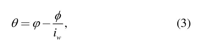
where iwis the transmission ratio of the vehicle’s steering system.

As shown in Fig.7,the scope of additional steer angles is±1.2°.It is clear that both the roll steer angle and the compliance steer angle do exist,and their absolute values grow greatly with the increasing of step steering angle.Due to the positive camber for both side wheels,the additional steer angles when turning left are greater than the values when turning right.

3.4 Effect of longitudinal acceleration and deceleration

When the vehicle accelerates or decelerates on a flat road,the whole mass of the vehicle will shift between front and rear axles,then the additional steer will be regarded as the compliance steer.The simulation tests were conducted under straight-line acceleration and braking conditions.

When the simulating was under the acceleration condition,the initial velocity was set as 20 km/h,and the gear at shift 2.At 1s after the beginning of simulation,the accelerating driving started.The simulation tests were conducted under different acceleration of 0.2g,0.3g,0.4g and 0.5g,respectively,and all the results are shown in Fig.8(a).We can see that with the increase of acceleration,the additional steer angle grows greatly,and at the acceleration of 0.5g,the compliance steer angle will be up to 0.3°(absolute value).

When the simulating was under the braking condition,the initial velocity was set as 120 km/h,and the gear at shift 5.The simulation tests were conducted on high adhesion coefficient road and the straight-line braking operation was employed.The braking started at 1s after the beginning of simulation.The simulations were conducted under different deceleration of 0.3g,0.4g,0.5g and 0.6g,respectively,and all the results are shown in Fig.8(b).We can see that the additional steer angle is within the range of±0.12°,and the greater the deceleration is,the larger the compliance steer angle will be.

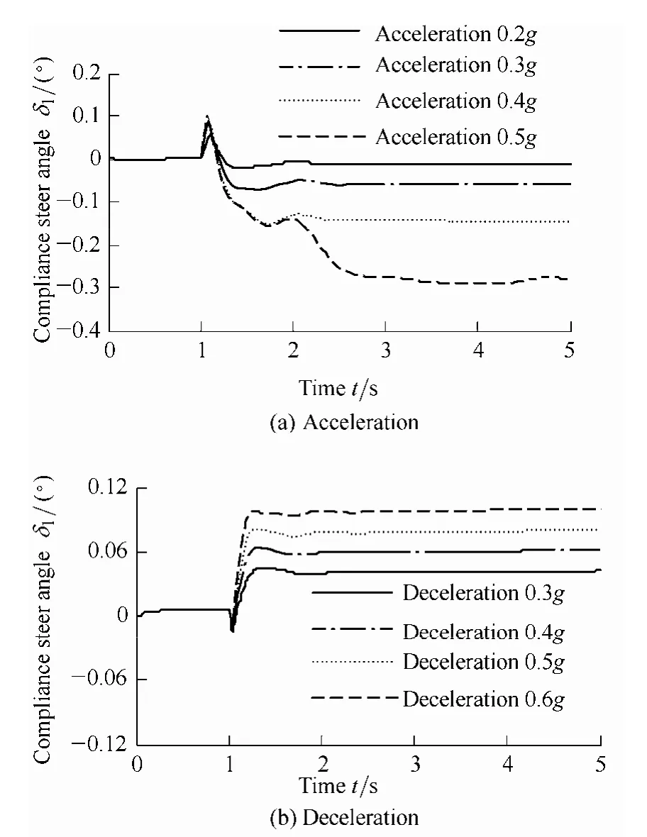
Fig.8.Compliance steer angle curves of left-front wheel caused by longitudinal acceleration and deceleration

Comparing Fig.8(a)with Fig.8(b),we find that the front wheel additional steer angle under deceleration is smaller than the angle under acceleration,which is related to suspension movement characteristics.Besides,while the value of left-front wheel additional steer angle is negative under the acceleration condition,the vehicle tends to turn right.However,under the braking condition,the vehicle tends to turn left.Thus,the influence of deceleration on vehicle's steering characteristics is contrary to the acceleration's.

4 Regression Model of Additional Steer Using Support Vector Machine

As analyzed above,the influence of lateral acceleration on the additional steer angle is maximal,which mainly depends on the steering angle of hand wheel and vehicle velocity,followed by the longitudinal accelerationdeceleration and the road wave amplitude,which are on the same magnitude.Other factor such as the longitudinal velocity has little effects on the additional steer angle and could be neglected.In general,vehicle dynamics control system only consider the relationship of additional steer angle with lateral acceleration,and neglects other factors,because the dynamic vehicle model can hardly be established accurately,especially under extreme driving conditions.Fortunately,the support vector machine(SVM)is particularly suitable for establishing this case of nonlinear mapping relationship.However,it is difficult to collect the samples and to select the algorithm to building the model meeting the requirements of real-time and control accuracy[11–12].

4.1 Determination of samples

In order to concretely quantify the additional steer angle under complex driving conditions,the input vector of the samples include vehicle longitudinal acceleration,lateral acceleration,yaw rate of body,displacement of suspension’s lower swing arm and steering angle of hand-wheel,while the output vector include only the additional steer angle.The displacement of suspension’s lower swing arm can indirectly reflect the changes of the road wave amplitude,so it is suggested that an acceleration sensor which is sensitive to the upward direction could be installed,and its output signals could be processed to obtain the displacement of sensitive direction.The method of FFT-DDI(fast Fourier transfer-digital double integration)is supposed to process the measurement data of acceleration sensor,in which the filtering of frequency domain and the integration of time domain are conducted alternatively.While conducting the filtering of frequency domain,the data of acceleration signal were firstly made FFT(fast Fourier transfer),then several front data and the last data of the FFT results are changed,so as to improve the integration accuracy for low frequency signal[13].All the other 4 input vector elements can be acquired from standard ESC configuration sensors.

Both learning samples and test samples were obtained from the slalom tests.These test data have covered the large steering angle of turning left and right,the big variation of vehicle lateral acceleration,yaw rate and suspension compliance,so they can reflect the additional steer angle responding to the input variation more effectively.The slalom tests are usually conducted on horizontal road,and the road wave amplitude is almost zero,but it will not affect the algorithm completion mentioned below.

The simulation driver files of slalom tests were created based on the ADAMS/Car simulation model built above.The slalom input steering was trigged from 1 s after the beginning of simulation.The maximal distance of the deviation from the center line in the slalom tests was 2 m.One of the driving curves of slalom tests is shown in Fig.9.

The samples were obtained by changing the deviation distance from the center line(such as 0.5 m,1 m,1.5 m,2 m)and velocity(such as 60 km/h,70 km/h,80 km/h,90 km/h,100 km/h).A row of data file representeda test point,totally 6 parameters.10 groups of different slalom tests data were selected randomly and processed as follows.The first lines of each data file were picked up and combined in order as the starting of a new learning sample.Then,the rest odd rows of each date file were picked up and appended sequentially in order as before.The test samples were determined using the even rows of any test file of slalom tests.Finally,the FMVSS 126 tests were supposed to conduct and create generalization test samples.All the samples should be normalized,because it could avoid the inconsistent contribution of different range of input elements to output accuracy,and improve the calculating speed simultaneously.

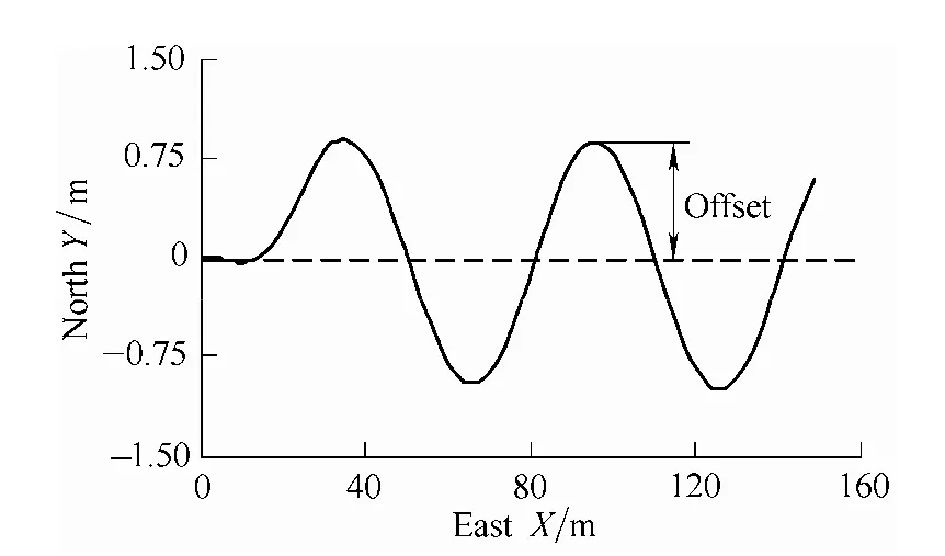
Fig.9.Driving curve of slalom test

4.2 Learning algorithm and optimization

We use the SVM toolbox LibSVM(Matlab version)to build the model to estimate the vehicle’s additional steer angle.LibSVM,developed by Professor Chih-Jen Lin,is a general software package of SVM,which provides five common kernel function of linear,polynomial,radical basis function,sigmoid and precomputed kernel.LibSVM is widely used in classification(including C-SVC and ν-SVC),regression(including ε-SVR and ν-SVR)and estimation of distribution(one-class-SVM)[14].

The LibSVM toolbox was firstly installed on Matlab platform,and the function svmtrain was used to train the samples to obtain the regression model of additional steer angle.Then the function svmpredict was recommended to get the estimated value by inputting the test samples to the regression model.Finally,the comparison between the estimated value and output element of test samples was made to determine the accuracy of regression model and whether the model parameters need to be adjusted again.In this paper,the ε-support vector regression(ε-SVR)algorithm was employed,and its kernel function was determined as RBF(Gaussian radial basis function),i.e.,

where X is the input vector of samples;Xcis the center vector of kernel function;σis the width parameter of kernel function,which controls the function radial scope,and the greater the value is,the wider the Gauss filter frequency scope will be.

In the ε-SVR algorithm,ε reflects the deviation between estimated values and sample values.The more the value ε is,the less the number of support vectors is required.As a result,the higher real-time model could be achieved.In addition,the penalty coefficient C and Gaussian radial basis function parameter σ also have a great effect on learning speed and estimation accuracy.The determination of value εdepends on actual application goals,while C and σ can be optimized using grid-search and crossvalidation method.

Table 2 shows the performance indexes of ε-SVR algorithm obtained from simulation tests.For a given ε,the optimal parameter group(C,σ)was obtained as follows.Firstly,a two-dimensional grid plane was determined based on the scope of parameters C and σ.For each cross point of the grid plane,the learning error of the additional steer angle was calculated using least squares support vector machine(LS-SVM).Finally,the parameter group with the minimal learning error was optimal.The PC’s timer method was employed to determine the SVM model prediction time-consuming on MCU,where the difference of these two CPU’s main frequency was considered.The MCU’s main frequency was 200 MHz,but the PC’s 1.6 GHz.The timing error of Windows operating system used on PC was more than 5 ms.In order to reduce the impact of timer error,the average value of 10 tests was resorted to determine the prediction time-consuming and each test was composed of 2 000 times continuous prediction for the same input vector.As shown in Fig.10,the curves were fit very well when ε is 0.1°.

Fig.10.Prediction example of additional steer angle of left-front wheel

As shown in Table 2,with the decrease of ε,the squared correlation coefficient of estimated curve with sample curve firstly increases and then decreases,but square errors firstly decreases and then increases.When ε equals to 0.1°,both of them achieve the peak value,and the regression effect is the best.However,the smaller the ε is,the more the support vectors will be required,so the estimation algorithm will consume longer time.When ε was bigger than 0.005°,the calculation time of MCU with 200 MHz main frequency will be less than 2 ms,which has met the real-time control requirements.

4.3 Model test of generalization ability

In order to verify the model generalization ability,the FMVSS 126 simulation tests were conducted using ADAMS/Car simulation model built above.The FMVSS 126 is a rules and regulations for ESC drawn up by NHTSA of USA in 2007[15].It is similar to the slalom test,and can reflect effectively the variations of each influencing factor on additional steer angle.The input vectors to the model were determined as section 4.2,and the prediction results were compared with the sample data to analyze the model generalization ability.

During the simulation tests,the vehicle was driven straight on the high adhesion road at the initial velocity of 80 km/h.The vehicle was subjected to use a steering pattern of a sine wave at 0.7 Hz frequency with a 500 ms delay beginning at the second peak amplitude.The peak of sine wave was determined as 1.5δ,2δ,3δ,4δ,5δ and 6δ,respectively.δ was determined by the slowly increasing steer test,in which the simulation model was run at the velocity of 80 km/h and the steering angle was increased by 13.5(°)/s until the lateral acceleration of approximately 0.5g was obtained.δ was the steer angle of hand wheel for this moment,and was about 30° for the simulation vehicle[7].Fig.11 shows the histories of the steering angle of hand wheel and the yaw rate of vehicle at the peak of sine wave 2δ,4δ and 6δ,respectively.

The samples for generalization ability testing employed the same normalization coefficients of the model learning samples.Table 3 shows the generalization results of the FMVSS 126 tests when ε equals to 0.1°,and(C,σ)(32,0.125).When the peak value of steering angle of hand wheel(δp)was 150°,the mean square error(MSE)is close to the minimum 0.071 6,meanwhile the squared correlation coefficient is maximal.In terms of MSE,the more the peak value δpis,the less the MSE is.Because the nonlinear degree of the whole vehicle increases with the increasing δp,and the learning samples were achieved under large nonlinear driving condition,the better prediction effect should come into being on the condition of big δp.Thus,it could be drawn that this support vectors regression model is highly adapted to the FMVSS 126 tests in prediction of the additional steer angle.Fig.12 shows the additional steer angle prediction curve of left front wheel in FMVSS 126 test when δpis 150°.

Fig.11.FMVSS 126 simulation tests

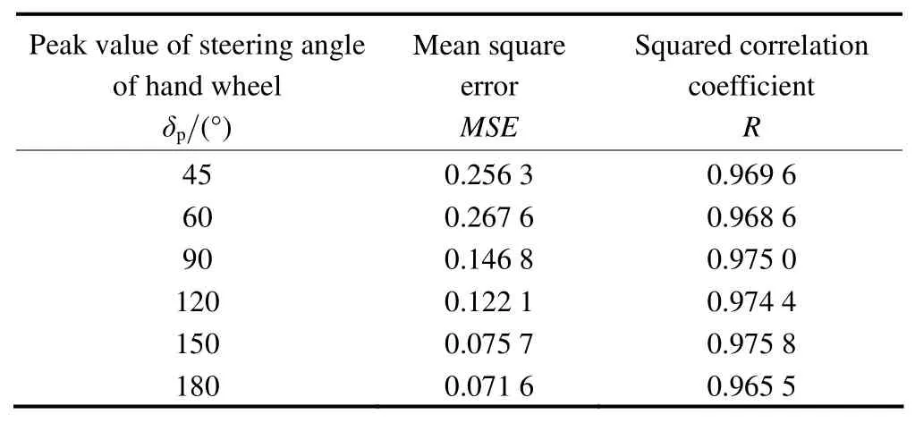
Table 3.Results of generalization test ε=0.1°,(C,σ)=(32,0.125)

Fig.12.Additional steer angle prediction curve of left-front wheel for FMVSS 126 test(δp=150°)

5 Conclusions

(1)An experimental observation method for the additional steer angle is brought forward and verified based on the simulation tests and the SVM model.It has expanded the accurate observation methods of the additional steer angle under extreme driving conditions.

(2)The quantitative analysis shows that the influence of lateral acceleration on the additional steer angle is maximal(the magnitude up to 1°),followed by the longitudinal acceleration-deceleration and the road wave amplitude(the magnitude up to 0.3°).Other factor such as the single longitudinal velocity has little effects on the additional steer angle and can be neglected.

(3)The input parameters of the SVM model are mainly composed of the standard configuration sensors signals of ESC.The results of both the slalom tests and the FMVSS 126 tests show that the prediction accuracy and the calculation time-consuming of the model can meet the requirements of ESC real-time control.

[1]VAN ZANTEN A T,ERHARDT R,PFAFF G,et al.Control aspects of the Bosch-VDC[C]//International Symposium on Advanced Vehicle Control,Aachen,Germany,June 24–28,1996:576–607.

[2]MITSCHKE M,WALLENTOWITZ H.Vehicle dynamics[M].4th ed.Beijing:Tsinghua University,2009.(in Chinese)

[3]LI Liang,LI Hongzhi,ZHANG Xiaolong,et al.Real-time tire parameters observer for vehicle dynamics stability control[J].Chinese Journal of Mechanical Engineering,2010,23(5):620–626.

[4]FUKAD Y.Slip-angle estimation for vehicle stability control[J].Vehicle System Dynamics,1999,32(4–5):375–388.

[5]KIN K,YANO O,URABE H.Enhancements in vehicle stability and steerability with slip control[J].JSAE Review,2003,24(1):71–79.

[6]BOADA B L,BOADA M J L,DÍAZ V.Fuzzy-logic applied to yaw moment control for vehicle stability[J].Vehicle System Dynamics,2006,43(10):753–770.

[7]ZHANG Xiaolong,LI Liang,SONG Jian,et al.Performance test and data processing method for vehicle electronic stability control system[J].Transactions of the Chinese Society for Agricultural Machinery,2011,47(5):1–6,34.(in Chinese)

[8]LI Liang,SONG Jian,LI Hongzhi,et al.A variable structure adaptive extended Kalman filter for vehicle slip angle estimation[J].International Journal of Vehicle Design,2011,56(1–4):161–185.

[9]HARADA M,HARADA H.Analysis of lateral stability withintegrated control of suspension and steering systems[J].JSAE Review,1999,20(4):465–470.

[10]HE Yuanchao.Research for the method of the key parameter selection in dynamics stability control logic[D].Beijing:Tsinghua University,2010.(in Chinese)

[11]ZHANG Xiaolong,LI Liang,LI Hongzhi,et al.Experimental research on vehicle sideslip angle estimation based on improved RBF neural networks[J].Journal of Mechanical Engineering,2010,46(22):115–110.(in Chinese)

[12]SUYKENS J A K,VANDEWALE J.Least squares support vector machine classifier[J].Neural Processing Letters,1999,9(3):293–300.

[13]RIBEIRO J G T,CASTRO J T P,FREIRE J L F.New improvements in the digital double integration filtering method to measure displacements using accelerometers[C]//Proceedings of the 19th International Modal Analysis Conference(IMAC XIX),Orlando,Florida,USA,February 5–9,2001:538–541.

[14]HSU Chih-Wei,CHANG Chih-Chung,LIN Chih-Jen.A practical guide to support vector classification[EB/OL].[2012-12-08].http://www.csie.ntu.edu.tw/～cjlin.

[15]U.S.Department of Transportation,Federal Motor Carrier Safety Admininstraton.Standard No.126,Electronic stability control systems[EB/OL].[2013-3-10].http://www.fmcsa.dot.gov/rulesregul-ations/administration/fmcsr/fmcsrruletext.aspx?reg=571.126.