
Different discretization method used in coupled water and heat transport mode for soil under freezing conditions
2013-10-09 08:11WeiNanMaoJianKunLiu
WeiNan Mao, JianKun Liu
School of Civil Engineering, Beijing Jiaotong University, Beijing 100044, China
1 Introduction
The freezing process of soil is a complicated comprehensive physical, chemical, thermodynamical and mechanical problem involved in the interaction among temperature, moisture and stress field. There are three main phenomena in the soil freezing process: moisture migration and phase change of water (the formation of ice crystals); heat transfer; the change of solute content.These three are mutual dependent, constraint, influenced,and the freezing process is a coupling change of those three (Maoet al., 2006; Liuet al., 2010). There are basically two kinds of coupled water and heat transport models used to describe the freezing process of soil (Zhuet al., 2007): model based on the viscous flow of liquid water in porous media and heat balance principle; model based on the description of water and heat flux by the application of irreversible thermodynamic theory.
In the early 1970s, Harlan (1973) proposed the concept of coupling hydrothermal and mathematical models for the freezing process and gave a numerical model,which is referenced by numerous scholars. Celiaet al.(1990) put forward an unsaturated water flow equation based on Richards equation. Liu and Guo (2011) analyzed the influence factors of heat and water migration in permafrost regions, discussed the heat and water migration research methods of frozen soil, established a coupled heat and water model considering the phase change of latent heat and soil freezing ice content, and a numerical solution was put forward. In addition, the studies of the phenomenon of soil freezing process also obtained a large amount of experimental data of water and heat coupling migration in the frozen soil (Du, 2012), which provides a solid foundation for the theoretical study.However, a more suitable coupling model using frozen soil and corresponding calculation software is urgently needed considering the fact that most scholars are still using unsuitable software for frozen soil. A new coupling model based on one dimension Richards equation used for unsaturated soil will be discussed in this work. Then,finite element and finite difference methods are applied in numerical calculations, respectively. At last, procedures of the aforementioned two kinds are used in simulating a freezing experiment.
2 Coupled water and heat transport mode for freezing
Hypothesis that the soil is incompressible, homogeneous and isotropic is applied in water migration problems. Soil moisture migration is similar to unsaturated soil water movement (Spaans and Baker, 1996). Adding the part of unfrozen water content change in an infinitesimal body at the same time, an improved Richards equation considering the phase change (Van Genuchten, 1980) can be written as(downwards ofzaxis is positive):
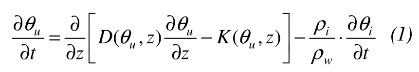
whereθiis ice content (cm3/cm3),ρiis ice density (0.917 g/cm3),ρwis the water density (1 g/cm3),Dis moisture diffusion coefficient in soil (cm2/s), andKis water conductivity in soil (cm/s).
When considering heat conduction in the frozen soil, latent heat can be recognized as an internal heat source. The balance equation for soil freezing can be given as:

whereCis heat capacity of soil [J/(cm3·K)],Tis temperature(K),λis coefficient of thermal conductivity of soil[W/(cm·K)], andLis latent heat (J/m3). There are many factors affectingCandλ, based on the research of Chenet al.(2011), the unfrozen water content can be the only considered affecting factor.
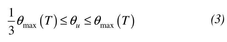
The factors in Equations(1)and(2)changed with the unfrozen water content, thus another contact relation must be brought in to solve the equations. The relationship curve between unfrozen water content and temperature is used.There are numerous researches on this relationship (e.g.,Chenet al., 2006), and some experience curves are given.An experience range between two curves based on the test result of silt clay is given. The top and bottom curves are determined by test data.
3 Finite difference numerical model
It is difficult to solve the coupled equation by analytical and semi-analytical methods because of nonlinearity. A numerical calculation method has proved to be appropriate in this situation. Leiet al. (1988) proposed a finite difference model used to solve similar equations.Unfortunately the implicit difference method is relatively complicated as well as temperature and hydraulic gradient have no clear physical meaning, at the same time the calculation accuracy has no obvious improvement. The model will be modified to solve the equations in a simple way.
Taking the temperature conduction equation for example, the heat transfer coefficient is related to its positionx. Equation(2)can be rewritten as:

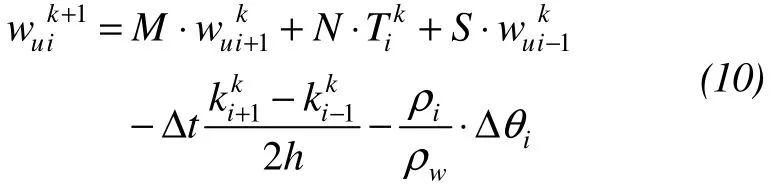
Using central difference in space coordinates and forward difference in time coordinates, for any pointiat any timek, Equation(4)can be written as:

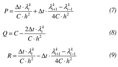
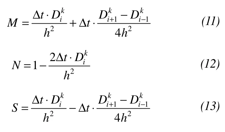
wherehis distance between adjacent nodes, and Δtis the interval time step, so the temperature of the next time is:
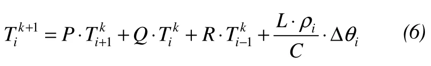
where,
whereiθΔ is change of ice content corresponding tok.
Similarly, the unfrozen water content of next time step is:
where,
Iterative calculation of each time step can be done according to the following procedure:
1) Forecast the temperature at the end of stepTk+1,Tkcan be determined approximately.
2) Adjust the unfrozen water content using Equation(3). If the unfrozen water content is out of the permitted range, the exceed part is the ice change at the end of this period of time.
3) Solve Equation(10)and obtain the unfrozen water content of each node at the end step.
4) Solve the heat flow equations and obtain the temperature of each node at the end of stepTk+1, which is the correction value of iterative calculation and the forecast value of next iterative calculation.
5) Repeat the steps above, till the unfrozen water content and temperature error between the last two steps are permitted.
6) RecalculateC,λandDusing the unfrozen water content and temperature produced in step 5. Repeat steps 1–5.
4 Finite element numerical model
Under one-dimensional condition, finite element is linear, for any point, temperatureTxcan be written by the node values and shape function:
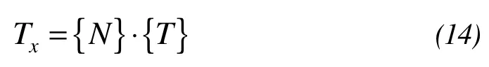
Substitute Equation(14)into Equation(2):

Use the Galerkin method to discrete Equation(15):
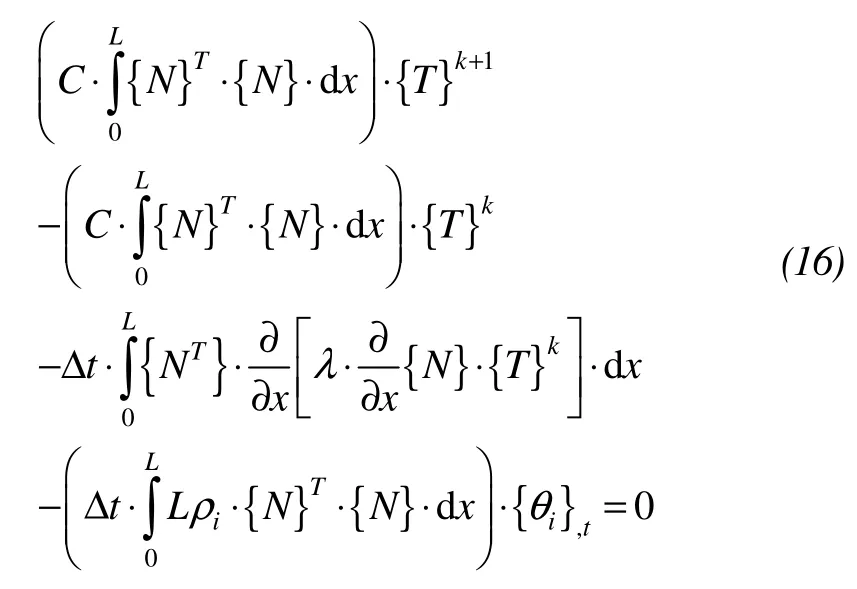
where Δtis the time interval. Equation(16)can be rewritten as:
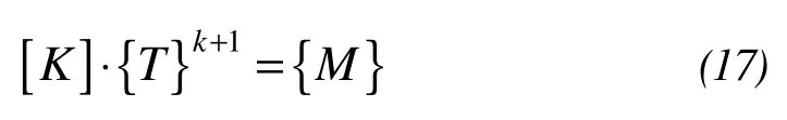
where,
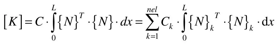
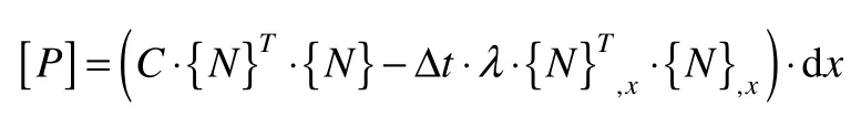
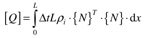
Solving Equation(17)we obtain the temperature of each node of the next step. The water calculation equation is:

Equations(3),(17), and(18)are the calculation equations for finite element numerical model. Calculation step part 3 can be used.
5 Experimental simulation
Two programs using FORTRAN language are written respectively, which are used to simulate the indoor experiment (Du, 2012). Silt clay soil is used for the one-way frozen experiment. The soil column diameter is 150 mm, height is 100 mm. The initial temperature of the soil is 1 °C. When the freezing starts, the top temperature is set to -2.5 °C and the bottom temperature is 1 °C. The initial water content is 0.15. There is a water filling bottle connected to the bottom of the sample.
The conductivity and diffusion coefficient of soil freezing can be obtained according to the values of unfreezing state (Leiet al., 1988):

whereθis total water content.
The soil thermal parameters can be given as (Leiet al.,1988):
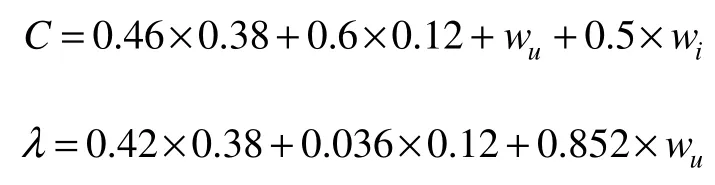
whereρiis 0.917 g/cm3,ρwis 1 g/cm3, andLis 335 J/cm3.
The filling bottle connected to the sample at the bottom nod is given a water content of 0.1, which is the average water content measured near the bottom during the whole experiment.
Variation of freezing depth during the whole experiment and the simulation results are presented in Figure 1.It shows that the error of finite element result is 0.5 cm larger than that of finite difference result and the frozen depth of finite difference result is 0.3 cm larger than the experiment value. Figure 2 shows the variation of freezing rate during the experiment and the simulation results,the curves of both different methods all tend to overlap the experiment curve. As is shown, the two numerical models can describe the freezing process very well.
Figure 3 shows the variation of temperature with depth at different times. The two curves of the two different meth-ods are approximately coincident, so there is only one simulation curve that can be seen in the figure. We can see the distribution of temperature at different moments of the soil sample from the contrast between simulation and the experimental result. The distribution curve is an exponential curve at the beginning of the experiment and changes to a quadratic parabola at the middle of the experiment; finally the temperature becomes steady and almost linear. The simulation results are smaller than the experiment result in the early (10 h) time, and coincident with the experiment result at about 20 h. In this period the results are the most accurate.The simulation values are greater. As mentioned above, the simulation freezing depth are deeper, these two are identical with each other.
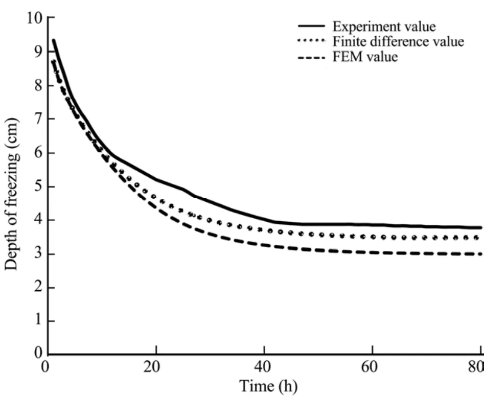
Figure 1 Variation of freezing depth
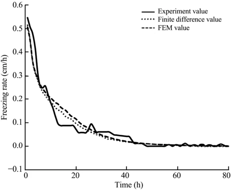
Figure 2 Variation of freezing rate

Figure 3 Variation of temperature
6 Conclusion
The interaction between temperature and water during soil freezing process is a complex problem in physics, chemistry,thermodynamics and mechanics. The established coupling model is based on full consideration of the interaction which well describe the freezing process, using finite different numerical method and finite element method in discretization;finally the two calculation programs are obtained. In simulation research, the result of one-dimensional model provides reference for the two-dimensional model in the future.
The authors wish to acknowledge the support and motivation provided by National 973 Project of China (No.2012CB026104), and National Natural Science Foundation of China (No. 41171064).
Celia MA, Bouloutas ET, Zarba RL, 1990. A general mass-conservative numerical solution for the unsaturated flow equation. Water Resour. Res.,26: 1483–1496.
Chen XB, Liu JK, Liu HX, Wang YQ, 2006. Frost Action of Soil and Foundation Engineering. Sciences Press, Beijing.
Du Y, 2012. Study on the Deformation Characteristics of 109 National Superhighway’s Sandy Silt Roadbed Fillings under Dynamic Load Action.Doctor’s Dissertation, School of Civil Engineering Beijing Jiaotong University, Beijing.
Harlan RL, 1973. Analysis of coupled heat-fluid transport in partially frozen soil. Water Resour. Res., 9: 1314–1323.
Lei ZD, Yang SX, Xie SC, 1988. Soil Hydrodynamic. Tsinghua University Press, Beijing.
Liu C, Chen XF, Yuan J, Li XY, 2010. Numerical simulation of coupled water and heat transportation in soil under freezing conditions. Water Resources and Power, (5): 94–96, 119.
Liu XY, Guo L, 2011. Analysis of the coupled water-heat soil temperature field in frozen sediment areas. Low Temperature Architecture Technology, (11): 87–88.
Mao XS, Li N, Wang BG, Hu CS, 2006. Coupling model and numerical simulation of moisture-heat-stress fields in permafrost embankment.Journal of Chang’an University (Nature Science Edition), 4: 16–19, 62.
Spaans EJA, Baker JM, 1996. The soil freezing characteristic: Its measurement and similarity to the soil moisture characteristic. Soil Sci. Soc. Am.J., 60: 13–19.
Van Genuchten MT, 1980. A closed-form equation for predicting the hydraulic conductivity of unsaturated soils. Soil Sci. Soc. Am. J., 44: 892–898.
Zhu Y, Chen XF, Ma W, Deng YS, 2007. Numerical simulation of water and heat transfer during unsaturated soil freezing. Anhui Agricultural Science,35(17): 5216–5217, 5282.
 Sciences in Cold and Arid Regions2013年4期
- Sciences in Cold and Arid Regions的其它文章
- Development of a dynamic load direct shear apparatus for the study of permafrost
- Roadbed, embankment, tower support and culvert stability problems on permafrost
- Field monitoring of railroad embankment vibration responses in seasonally frozen regions
- Reinforcement effects of ground treatment with dynamic compaction replacement in cold and saline soil regions
- Review of the influence of freeze-thaw cycles on the physical and mechanical properties of soil
- Neumann stochastic finite element method for calculating temperature field of frozen soil based on random field theory