Neumann stochastic finite element method for calculating temperature field of frozen soil based on random field theory

Tao Wang , GuoQing Zhou

1. State Key Laboratory for Geomechanics and Deep Underground Engineering, China University of Mining and Technology,Xuzhou, Jiangsu 221116, China

2. School of Architecture and Civil Engineering, China University of Mining and Technology, Xuzhou, Jiangsu 221116, China

1 Introduction

For frozen soil, the temperature field calculation is the basic problem for strength and stability. Because of the complexity of the analytical solution for the temperature field, the finite element (FE) method of numerical solution is widely popular with researchers. Traditional FE analysis of the temperature field generally does not consider the effects of random factors; all of the parameters in the study area are regarded as deterministic variables (Ge, 2008; Wang and Chen, 2008).

Geotechnical soil can form only after long geological time. Its composition is very complicated as a result of many natural and human factors. Therefore, the parameters of geotechnical soil have the characteristics of random distribution. Also, because of the particularities of the soils, the geotechnical parameter values obtained by geotechnical engineering tend to have great variability and uncertainty (Wanget al., 2009; Zhanget al., 2009). If random parameters are simulated as random variables in the process of calculation,the original deterministic temperature field analysis becomes uncertain temperature field analysis including random variables; this is called the random variable FE method.

Oktay and Kammer (1982) first took into account the randomness of the parameters in the temperature field.Madera and Sotnikov(1996) suggested a numerical method for computing the mathematical expectation and correlation distributions of a stochastic temperature field. After that, the random variable FE method was widely used to solve random temperature field problems (Liet al., 2007, 2009, 2010;Chenet al., 2009). Qiet al.(2005) calculated the random temperature field of frozen soil roadbeds in the Bailu River section of the Qinghai-Tibet Railway based on the first-order Taylor series expansion. Sunet al.(2011) calculated the random temperature field of a typical frozen soil roadbed by the Monte-Carlo stochastic FE method.

In a broad sense, an FE method is considered stochastic as long as it takes into account the random variables in the FE calculation. But Vanmarcke and Grigoriu(1983) and Vanmarckeet al.(1986) pointed out that the "true" random FE method must include handling of the random field. The randomness of soil parameters needs to be modeled as a spatially random field instead of a traditional random variable. To take into account the random field, discretization is necessary and this is called the random field FE method.Because the calculation of random temperature fields including random fields is unusual, there is less research on this aspect. Zhang and Li (1993) analyzed the random temperature and thermal stresses in concrete structures based on the theory of stochastic progress. Wanget al.(2003) combined the stochastic process theory with the thermal transfer theory and analyzed the influence of the random thermal shock impacts on the piston in a gas engine. Also, Xiu and Karniadakis (2003) and Emery (2004) gave the solution of stochastic heat transfer problems based on the theory of stochastic progress.

The stochastic process can be considered as a one-dimensional random field, but it is different with a two-dimensional random field and a three-dimensional random field. Liuet al.(2006) calculated the random temperature field of a frozen soil roadbed by the first-order perturbation stochastic FE method based on the local average theory of random field. However, a detailed description of the random field and numerical characteristics of the local average random field were not given, and the results obtained from the first-order perturbation stochastic FE method were not accurate when the perturbation was more than 20% to 30%.Using a second-order perturbation stochastic FE method would involve massive calculations and would thus be very time-consuming. Therefore, a more efficient and more accurate method is needed to calculate the random temperature field of frozen soil, and the objective of this paper is to introduce such a method.

By modeling the heat transfer coefficient and specific heat capacity as a spatially continuous stationary random field, a series of local average random fields can be obtained based on the discrete theory of the local average theory of random fields. Combining elements of local average random fields with FE element, we calculated the random temperature field of seasonal frozen soil by the Neumann stochastic FE method. Based on the calculation flow chart, the stochastic FE calculation program for solving the random temperature field was compiled by MATLAB (MathWorks, Inc.,Natick, Massachusetts). An example is presented here to demonstrate the feasibility and effectiveness of this method.

2 Transient heat conduction problems

2.1 Heat conduction equation

For the 2D heat conduction problem of the temperature field, the basic equation can be written as:

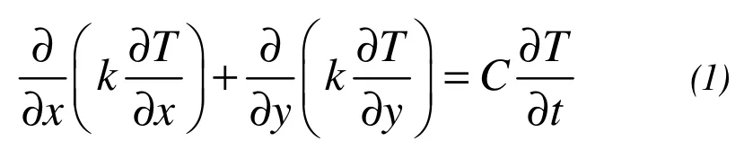
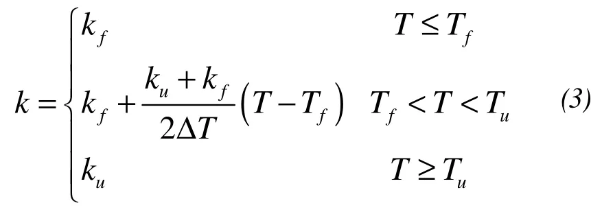
whereTis the temperature,tis the time,Cfis the specific heat capacity of frozen soil,Cuis the specific heat capacity of unfrozen soil,Lis the latent heat of phase transition, ΔTis temperature range of the phase transition,kfis the heat transfer coefficient of frozen soil,kuis the heat transfer coefficient of unfrozen soil,Tmis the mean temperature of phase transition, and (x,y) is the position coordinate.

2.2 Boundary conditions

There are three kinds of common boundary conditions in the heat transfer problems. The first is:

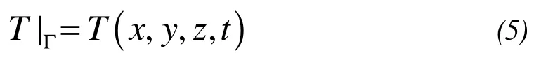
whereΓis the boundary surface.

The second is:

wherenis the external normal direction,andqwis the heat flux.

The third is:

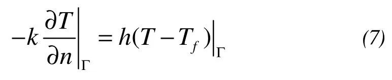
wherehis the surface heat transfer coefficients,andTfis the temperature of the gas flow .

2.3 Initial conditions

In order to obtain the solutions of Equation(1), the initial conditions are:

wheret0is the initial timeandT0is the initial temperature field.

3 Finite element equations

The FE equations of the temperature field based on the FE method is:

where [K] is the stiffness matrix of temperature,[N] is the unsteady temperature matrix, {T}tis the column vector of temperature, {P}tis the right column vector, andtis the same time of every column vector.

Based on the backward difference method, Equation(9)can be written as:

where Δtis the time step.

When solving the {T}tas long as {T}t-Δtis known, Equation(10)can be simplified as:

where

BothKandRare deterministic variables in the traditional deterministic FE method, soTof Equation(11)is a deterministic result. The random variable FE method models the heat transfer coefficient and specific heat capacity as random variables. That is to say, bothKandRare random variables, soTof Equation(11)is also a random result. But Vanmarcke (1977) pointed out that the variability of spatially random parameters is not accurately described by the random variables method. The variability of spatially random parameters needs to be modeled as spatially random fields. The main objective of this paper is to calculate the random temperature field by modeling the heat transfer coefficient and specific heat capacity as a spatially continuous stationary random field.

4 Local average methods of the random field

At present, both spatial discretization and abstract discretization can approximately describe the random fields.Spatial discretization methods include the central discrete method, the local average method, the interpolation method,the local average method, the local integral method and the orthogonal expansion method. Abstract discretization methods include the decomposition method of Karhumen-loeve and the orthogonal series expansion method. The methods of spatial discretization can use many of the basic relations of the FE method, but the methods of abstract discretization cannot use them; a large amount of programming work is necessary to modify the FE method program (Qin, 1994). In view of this, this paper uses the local average method to discretize the random field because it converges rapidly, has high precision, and it needs less statistical information than the other methods.

4.1 Discretization

The accuracy of calculation results for the random temperature field depends on the grids of the FE mesh and the random field mesh. The size of the FE mesh relates to the temperature gradient, and the size of the random field mesh relates to the correlation distance (Vanmarckeet al., 1986).When the number of the FE mesh is too much, a random field mesh can be chosen which is different from the FE mesh. This is appropriate when the length of the random field element is one-third or one-half of the correlation distance, and it is also suitable when every element of the random field contains one or two finite elements (Liu PL and Liu KG, 1993). Assuming that the random field mesh has been divided; the random field of some parameterwould be divided into many random vectors. According to the characteristics of the continuous stationary random field, the mathematical expectation of the local average random field is equal to the original random field. The variances of the local average random field are the main elements of the covariance matrix. Therefore, the main work of the random field FE method is the calculation of the covariance matrix.

We modeled the heat transfer coefficient and specific heat capacity as a 2D continuous stationary random field.ξ(x,y) is a random variable of a physical parameter in a certain position. {X(x,y), (x,y)∈R2} constitute a 2D continuous stationary random field. IfE[X(x,y)] =mandVar[X(x,y)] =б2, the mathematical expectation, variance and covariance of{Y(x,y)=X(x,y)-m, (x,y)∈R2} are:

Therefore, it is without loss of generality when we assume that the mean function is zero for the analysis of the numerical characteristics of the local average random field.

4.2 Numerical characteristics of the quadrilateral element of the local average random field

X(x,y) is a 2D continuous stationary random field. The mathematical expectation is zero and the variance is constant.That is to say,E[X(x,y)]=m=0 andVar[X(x,y)]=б2. The random field mesh of the arbitrary quadrilateral element is shown in Figure 1.

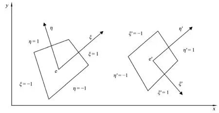
Figure 1 Two-dimensional arbitrary quadrilateral element of a local average random field

The local average random field of an element is defined as:

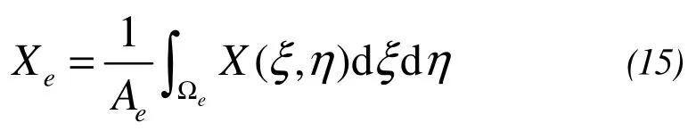
whereAeis the area ofeand Ωeis the possessive section ofe.

The mathematical expectation and covariance of the local average random field of an element are:

where

whereAeis the area ofe,Ae'is the area ofe′.ρ(r,s) is a standard relevant coefficient,Niis the shape function ofe,Ni′is the shape function ofe′,xiandyiare the position coordinates ofe,xi′andyi′arethe position coordinates ofe′,(ξ,η)and (ξ′,η′) are the local position coordinates.

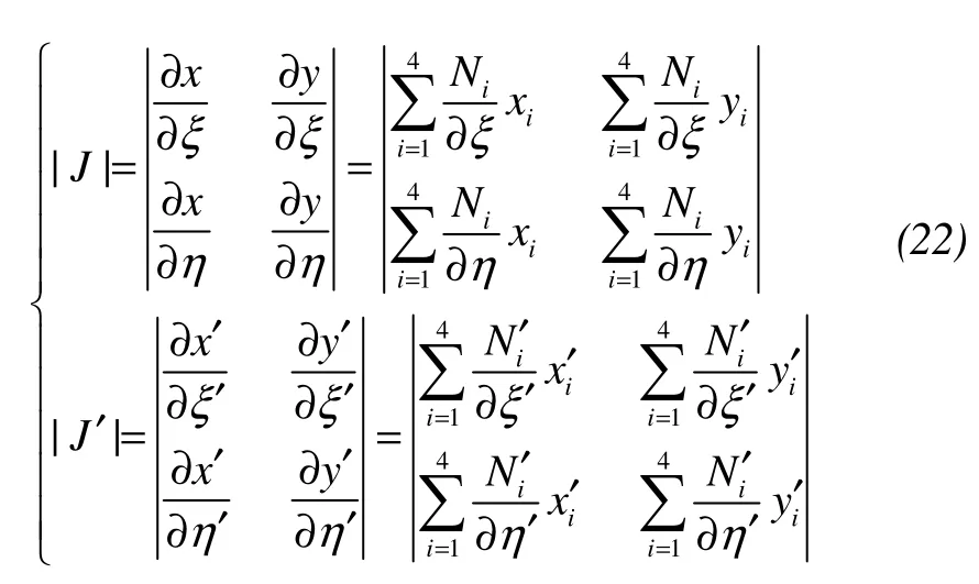
where |J| and |J′| are the Jacobian determinants of coordinate transformation. In order to guarantee the correctness of the conversion, it needs |J|≠0 and |J′|≠0. That is to say, every interior angle of the quadrilateral element of the local average random field must be less than 180°.

It is difficult to obtain the explicit formulation of Equation(17), so we need the Gauss numerical method to perform the integration. Based on Gauss numerical integration method, Equation(17)can be rewritten as:

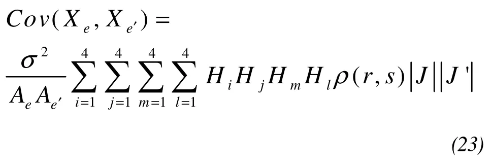
whereHi,Hj,HmandHlare the weighting coefficients.

4.3 Independent transformation of the local average random field

After discretization of the continuous stationary random field by the local average theory, the statistical characteristics of the random field can be approximately described by a series of mathematical expectations and covariances of random variables. Because covariance matrices are full-rank matrices, the computational load is heavy for a large number of random variables of complex construction. Therefore, in this paper, a set of uncorrelated random variables is obtained by independent transformation of correlated random variables based on the proper orthogonal transformation method.The covariance matrix obtained by the local average theory is a real, symmetric, positive, definite matrix. Its eigenvectors are real numbers based on the theory of eigenvalues and eigenvector of the matrix. Also, there areMlinearly independent eigenvectors for anMorder real symmetric matrix.

Assuming the zero mean random vectorαis (α1,α2, …αM)T, its covariance matrixAis [Cov(αi,αj)], the irrelevant random vectorβis (β1,β2, …,βM)T, its varianceBis diagonal matrix [Var(βi)]M×M, andPis the linear transformation matrix, there are:

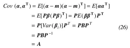
wherePis the eigenvector matrix ofA,Bis the eigenvalues matrix ofA,andmis the mean vector ofα.

Therefore, as long as unrelated normal random variables produced by MATLAB obey the normal distribution ofN(0,Var(βi)) for every element of the random field, the samples of discretization of the local average random field can be obtained by Equation(25).

5 Temperature field of frozen soil based on the Neumann stochastic FE method

The temperature field of frozen soil can be calculated by FE equations,boundary conditions and the samples of discretization of the local average random field based on the Monte-Carlo method. The Monte-Carlo method is accurate when the perturbations are more than 20% to 30%. It can be perfectly combined with the deterministic FE method and thus avoid the complicated theoretical derivation. However,there are many related random variables when the numbers of finite elements and random fields are large; calculating the inverse of the stiffness matrix of the temperature will require lengthy computation time for every FE analysis. In order to improve the efficiency of such a calculation, the Neumann expansion (Yamazakiet al., 1988) is used in this paper.

The random stiffness matrix of Equation(11)can be broken down into:

whereK0is the average temperature stiffness matrix of the random variables or the random field, andΔKis the undulatory section.

Only ΔKandRhave a change for every random sampling by the Monte-Carlo method. Based on the Neumann expansion, when ||K0-1ΔK||<1,

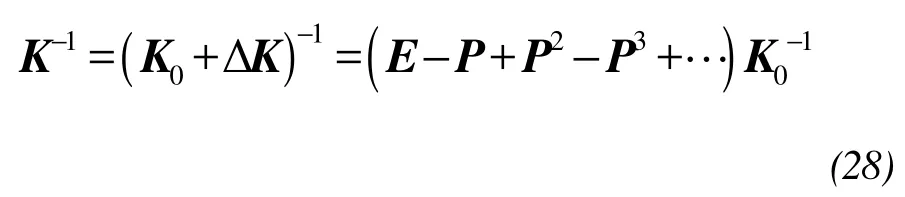
whereEis the unit matrix, andP=K0-1ΔK.

According to Equation(11), there is:

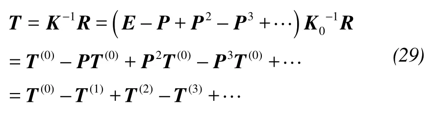
whereT(0)=K0-1R,T(i)=Pi T(0).

According to Equation(29), there is

Therefore, theT(0)can be acquired byT(0)=K0-1R, theT(1),T(2),T(3),…can be obtained from Equation(30), and theTcan be obtained from Equation(29). The truncation method is needed because Equation(29)is the infinite number of the matrix. In a general way, it is not necessary to calculateT(m+1)when|T(m)i-T(m-1)i|<εfor arbitraryi(1≤i≤M;Mis the number of FE nodes,εis the smaller values). The result is the sum of the first (m+1) items.

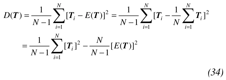
The mathematical expectation matrix, the variance matrix and the variable coefficient matrix can be obtained by statistical analysis of the temperatures of the FE nodes. The computational formulae are:

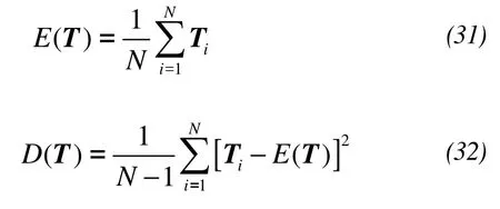
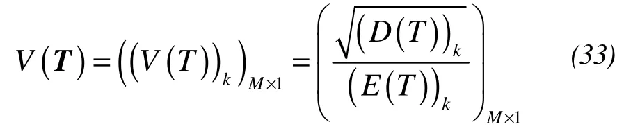
whereTiis the temperature array of the FE nodes that can be obtained at theitime calculation,Nis the number of times for random calculation, andMis the number of FE nodes.

In order to easily program the computer by MATLAB,according to the Equations(31)and(32), we can obtain:

Based on the above analysis, Figure 2 is the flow chart for calculating the random temperature field of seasonal frozen soil. As shown in the figure, the stochastic FE calculation program for solving the random temperature field was compiled by MATLAB.

6 Numerical examples

Figure 3 is the section shape of a geotechnical structure.For melted soil,ku=2,785.2 kJ/(m3·°C), andCu=2.18 W/(m·°C); for frozen soil,kf=1,994.8 kJ/(m3·°C), andCf=3.05 W/(m·°C). For the boundary of AB,qw=8 W/m2; for the boundary of CD and DA,TCD=-10 °C,TDA=5 °C; and BC is adiabatic. The initial temperature field is 15 °C. If we assume that all random parameters follow a normal distribution and their variable coefficients are 0.25. Table 1 presents the statistics of the thermal parameters, and Table 2 presents the statistics of the boundary conditions. The problem to be answered is how to obtain the statistical properties of the temperature field.

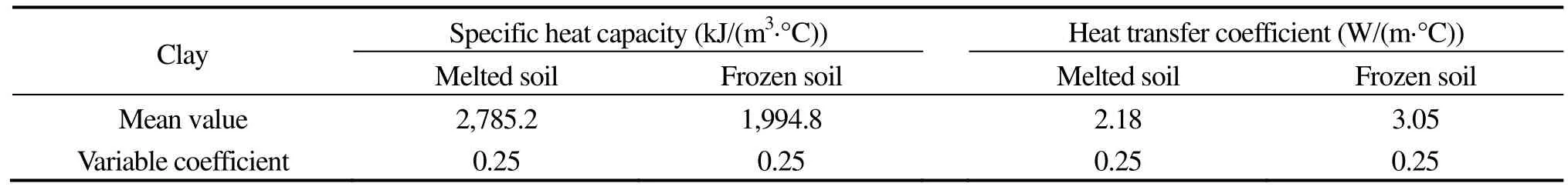
Table 1 Statistics of the thermal parameters

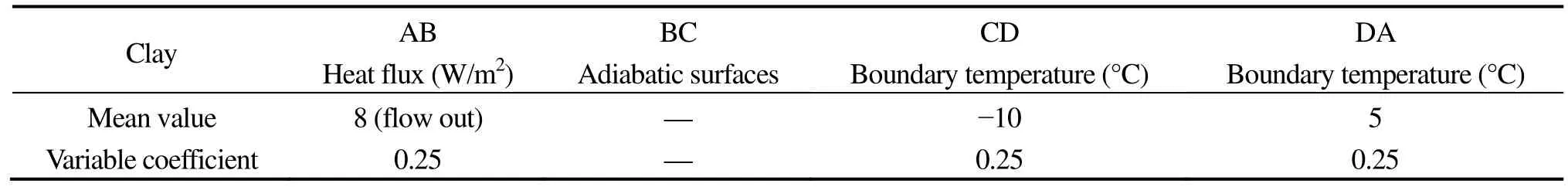
Table 2 Statistics of the boundary conditions

Figure 4 shows the mesh of the triangular elements based on the FE method. There are 310 elements and 181 nodes. We modeled the heat transfer coefficient and the specific heat capacity as continuous stationary random fields,and the heat flux density and the boundary temperature as random variables. Figure 5 shows the quadrilateral elements of the random field mesh. There are 150 quadrilateral elements and two different random fields. Therefore, there are 300 random variables. Comparing Figure 4 with Figure 5 indicates that every mesh of the local random field contains two or three meshes of finite elements. We assumed thatρ(r,s)=exp(-(r+s)/60) and randomly calculated 10,000 times by the stochastic FE calculation program. In order to make a comparative analysis, we analyzed the model that the heat transfer coefficient and the specific heat capacity are only dealt as random variables.

Figures 6a,b show the distributions of the mean temperature after one day, and Figures 7a,b show them after three days. It can be seen from Figure 6 that the mean temperature field distributions are roughly the same when the heat transfer coefficient and specific heat capacity are treated as random fields or random variables. A similar conclusion can be made from Figure 7.

To validate the method proposed in this paper, we calculated the temperature field based on the Monte-Carlo method. Figure 8 shows the distributions of the mean temperature after one day, and Figure 9 shows them after three days. It can be seen from Figures 6a and 8 that the mean temperature field distributions are roughly the same after one day, and from Figures 7a and 9 that the mean temperature field distributions are also roughly the same after three days. Therefore,the method proposed in this paper, the Neumann stochastic FE method based on random field theory, is reasonable and true. The same computer would spend 7,894.543 s by the method proposed here, and 9,876.423 s by the Monte-Carlo method. This proves that our method is more efficient.

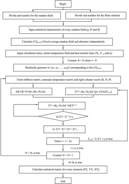
Figure 2 Calculation flow chart of the random temperature field

Figures 10a,b show the distributions of variance of the temperature field after one day, and Figures 11a,b show them after three days. It can be seen from Figure 10 that the variance obtained by the random field model is smaller than the variance obtained by random variable model at the same position of the section. A similar conclusion can be made from Figure 11. Therefore, we can conclude that modeling the random parameters as spatially random fields will reduce the variability of the temperature field. These results conform to the theoretical analysis because the variances of the local average random field are smaller than the original random field.

Figure 3 Cross section of the geotechnical structure

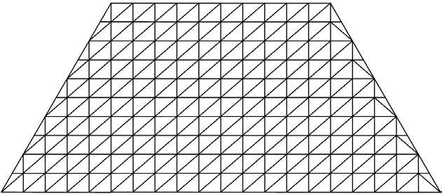
Figure 4 Finite element mesh

Figure 5 Random field mesh

Figure 6 Distribution of mean temperature based on the Neumann expansion method (°C, 24 h). (a) The heat transfer coefficient and specific heat capacity are modeled as random fields; (b) The heat transfer coefficient and specific heat capacity are modeled as random variables

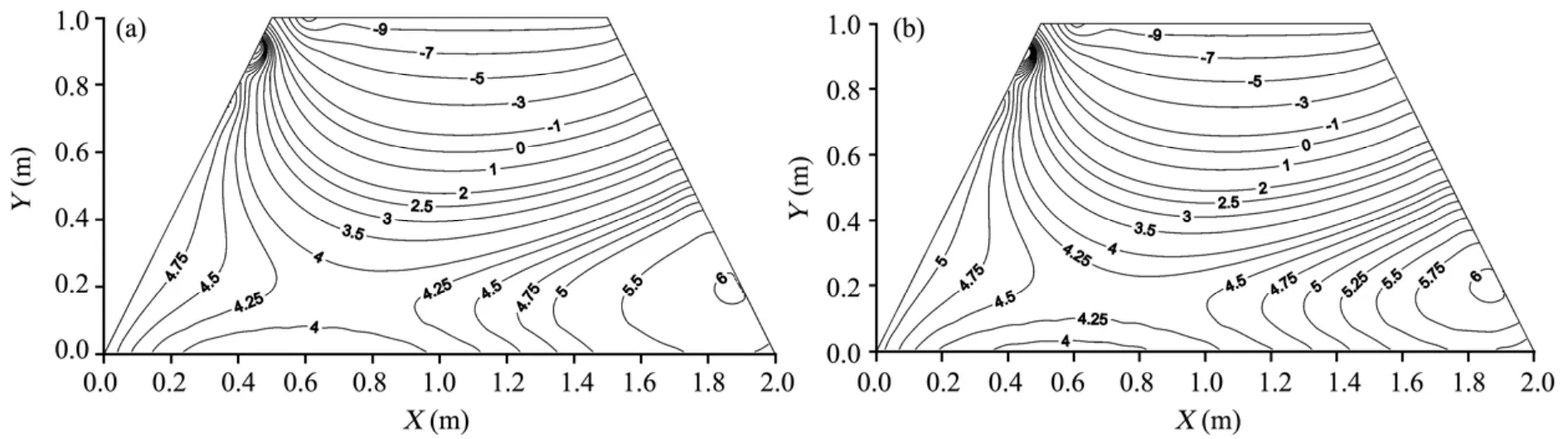
Figure 7 Distribution of mean temperature based on the Neumann expansion method (°C, 72 h). (a) The heat transfer coefficient and specific heat capacity are modeled as random fields; (b) The heat transfer coefficient and specific heat capacity are modeled as random variables

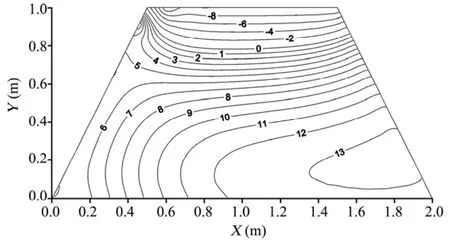
Figure 8 Distribution of mean temperature based on the Monte-Carlo method (°C, 24 h)

Figure 9 Distribution of mean temperature based on the Monte-Carlo method (°C, 72 h)

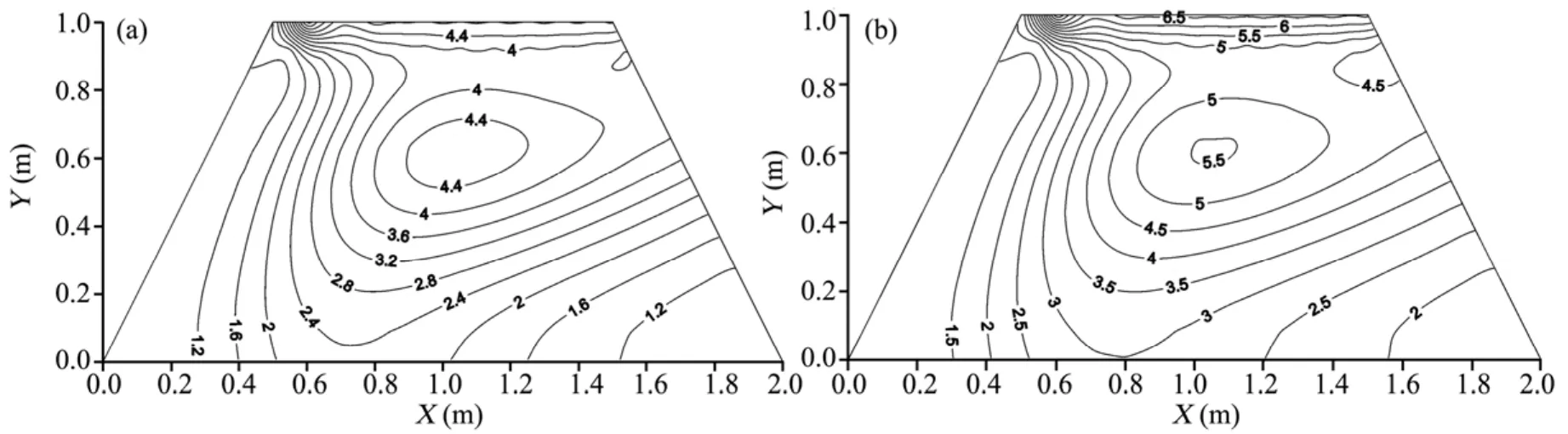
Figure 10 Distribution of variance based on the Neumann expansion method (°C2, 24 h). (a) The heat transfer coefficient and specific heat capacity are modeled as random fields; (b) The heat transfer coefficient and specific heat capacity are modeled as random variables

Figure 11 Distribution of variance based on the Neumann expansion method (°C2, 72 h). (a) The heat transfer coefficient and specific heat capacity are modeled as random fields; (b) The heat transfer coefficient and specific heat capacity are modeled as random variables

7 Conclusions and discussions

1) The Neumann stochastic FE method can efficiently solve problems about random temperature fields of frozen soil based on random field theory. It is accurate when the perturbations are more than 20% to 30% and can perfectly combine with deterministic FE method.

2) According to the calculation flow chart, the stochastic FE calculation program compiled by MATLAB can directly output the desired statistical results (the mathematical expectation matrix, the variance matrix, and the variable coefficient matrix [E(T),D(T), andV(T), respectively]) of the random temperature field.

3) Modeling the random parameters as traditional random variables will increase the variability of the temperature field. Therefore, modeling the random parameters as spatially random fields is accurate and necessary.

4) Using the Neumann stochastic FE method described in this paper, problems about the random temperature fields of multi-layer soil could be easily solved after making slight modifications.

Several concepts and methods related to using random field theory for calculating the temperature field of frozen soil has been introduced here. However, several issues still need to be addressed concerning the engineering applications of this method, such as moisture migration and the spatial variability of frozen soil. Therefore, many researches still need to be done in the future.

This research was funded by the National Basic Research Program of China (No. 2012CB026103), the National High Technology Research and Development Program of China(No. 2012AA06A401), and the National Natural Science Foundation of China (No. 41271096). We express our sincere thanks to the anonymous reviewers for their valuable comments and suggestions on the content of the paper and on the use of language.

Chen JJ, Wang LG, Li JP, 2009. Thermal response analysis of stochastic pole structures under steady random temperature field. Engineering Mechanics, 26(suppl. 1): 12–15.

Emery AF, 2004. Solving stochastic heat transfer problems. Engineering Analysis with Boundary Elements, 28(3): 279–291.

Ge JJ, 2008. Numerical simulation of the temperature regime within an embankment with insulated berm of the Qinghai-Tibet Railway. Journal of Glaciology and Geocryology, 30(2): 274–279.

Li JP, Chen JJ, Liu HF, Xu J, Huang XB, 2007. Analysis of stochastic temperature field by the Neumann expansions. Journal of Xidian University,34(3): 454–457.

Li JP, Chen JJ, Yue LJ, Liu GL, 2009. Analysis of temperature field with fuzzy-random parameters based on general density function. Journal of Wuhan University of Technology, 31(15): 115–144.

Li JP, Chen JJ, Zhu ZQ, Liu GL, 2010. Asymptotic-maximum entropy analysis of stochastic temperature field. Chinese Journal of Applied Mechanics, 27(1): 58–62.

Liu PL, Liu KG, 1993. Selection of random field mesh in finite element reliability analysis. Journal of Engineering Mechanics, 119(4): 667–680.

Liu ZQ, Lai YM, Zhang MY, Zhang XF, Lu H, 2006. Stochastic temperature field of frozen ground road-bed. Science in China (Series D), 36(6):587–592.

Madera AG, Sotnikov AN, 1996. Method for analyzing stochastic heat transfer in a fluid flow. Applied Mathematical Modelling, 20(8): 588–592.

Oktay S, Kammer HC, 1982. A conduction-cooled module for high-performance LSI devices. IBM Journal of Research and Development, 26(1): 55–66.

Qi CQ, Wu QB, Shi B, Xu HZ, 2005. Stochastic finite element analysis for the temperature field of frozen soil roadbed of Qinghai-Tibet Railway.Journal of Engineering Geology, 13(3): 330–335.

Qin Q, 1994. Progress in stochastic finite element methods, Part I. Discretization of random fields and moments of structural responses. Engineering Mechanics, 11(4): 1–10.

Sun H, Niu FJ, Chen Z, Ge XR, 2011. Stochastic temperature field of frozen soil roadbed based on Monte-Carlo method. Journal of Shanghai Jiaotong University (Science), 45(5): 738–742.

Vanmarcke E, 1977. Probabilistic modeling of soil profiles. Journal of the Geotechnical Engineering Division, 103(11): 1227–1246.

Vanmarcke E, Grigoriu M, 1983. Stochastic finite element analysis of simple beams. Journal of Engineering Mechanics, 109(5): 1203–1214.

Vanmarcke E, Shinozuka M, Nakagiri S, Schuëller GI, Grigoriu M, 1986.Random fields and stochastic finite elements. Structural Safety, 3(3–4):143–166.

Wang YZ, Hu YC, Hong RH, Yu ZT, Shen JS, 2003. Stochastic analysis of temperature for thermal shock on piston with lumped parameter model.Transactions of CSICE, 21(1): 81–85.

Wang SJ, Chen JB, 2008. Nonlinear analysis for dimensional effects of temperature field of highway embankment in permafrost regions on Qinghai-Tibet plateau. Chinese Journal of Geotechnical Engineering,20(10): 1544–1549.

Wang YH, Wang BT, An YY, 2009. Study of random field characteristics of soil parameters based on CPT measurements. Rock and Soil Mechanics,30(9): 2753–2758.

Xiu DB, Karniadakis GE, 2003. A new stochastic approach to transient heat conduction modeling with uncertainty. International Journal of Heat and Mass Transfer, 46(24): 4681–4693.

Yamazaki F, Shinozuka M, Dasgupta G, 1988. Neumann expansion for stochastic finite element analysis. Journal of Engineering Mechanics,114(8): 1335–1354.

Zhang DX, Li ML, 1993. Analysis of random thermal stresses of concrete slabs restricted on elastic bases. Journal of Tongji University, 21(1):91–97.

Zhang JZ, Miao LC, Wang HJ, 2009. Methods for characterizing variability of soil parameters. Chinese Journal of Geotechnical Engineering, 31(12):1936–1940.