Optimal quasi-periodic maintenance policies for two-unit series system
Gao Wenke Zhang Zhisheng Zhou Yifan Gan Shuyuan
(School of Mechanical Engineering, Southeast University, Nanjing 211189, China)
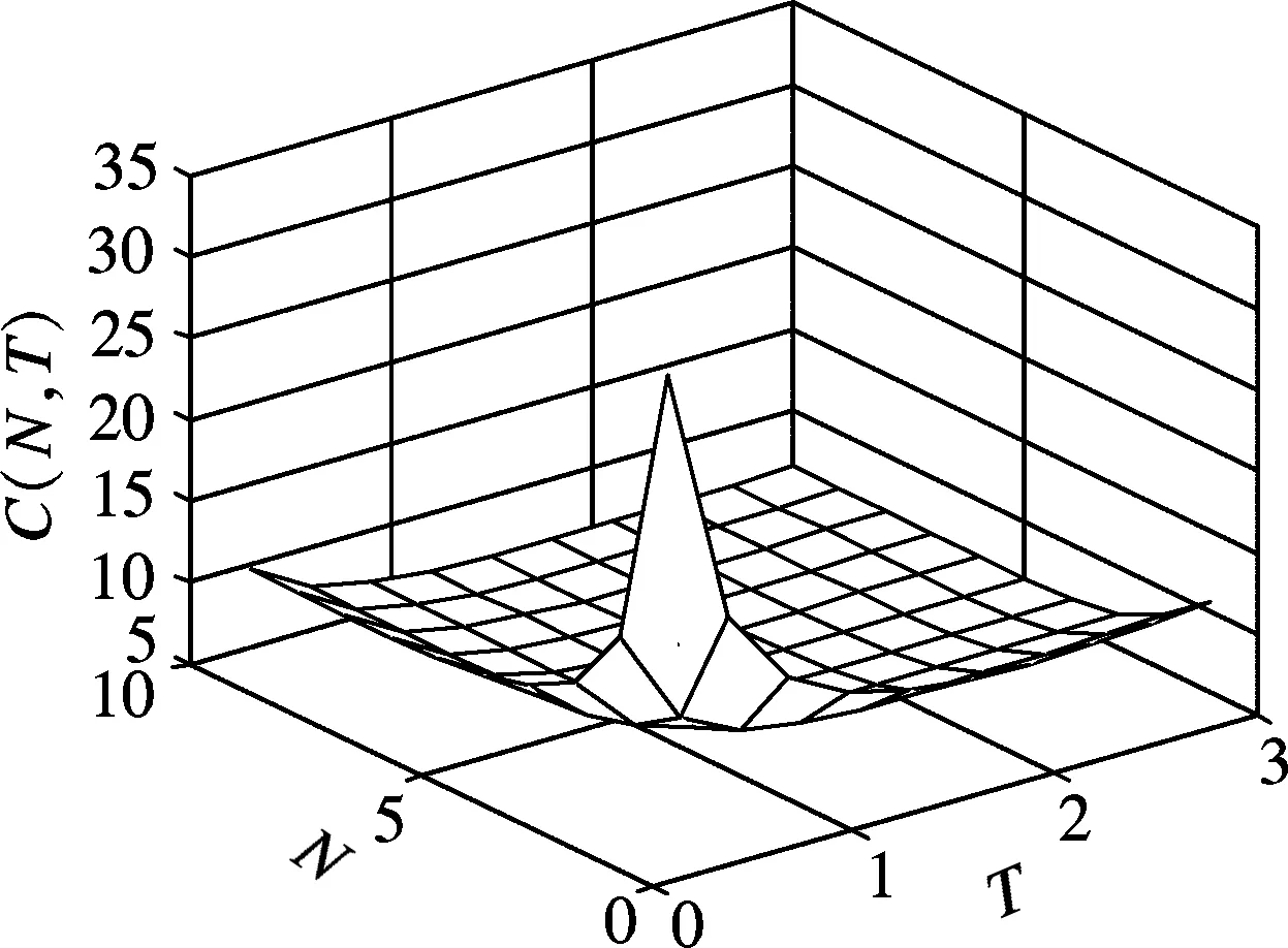
As one of some major maintenance policies, preventive maintenance (PM) policy is widely used to reduce downtime and breakdown risk in areas such as industry, military, health and the environment. As such, the effective implementation of PM policies has been extensively studied[1]. Most research on PM models is concerned with the optimal maintenance policies for a machine or a mono-unit system[2]. In contrast, the PM models of two-unit systems have received less attention, and many of these existing works focused on redundant systems[3-4]or condition-based maintenance[5]. However, one type of two-unit series system is broadly existent in practice, in which the lifetime of unit 1 (U1) is always stochastically much smaller than that of unit 2 (U2), and PM forU1is nearly perfect while forU2is only mechanical service and the system will be replaced if a catastrophic failure ofU2occurs, for example, a cylinder and its cylinder liner, a nozzle matching parts of a diesel engine, plunger matching parts, and so on. Meanwhile, PM plans of the system are often modified by some random factors, such as production task, the transport cycle of a locomotive, which make the PM intervals become a limited stochastic value rather than a fixed value.
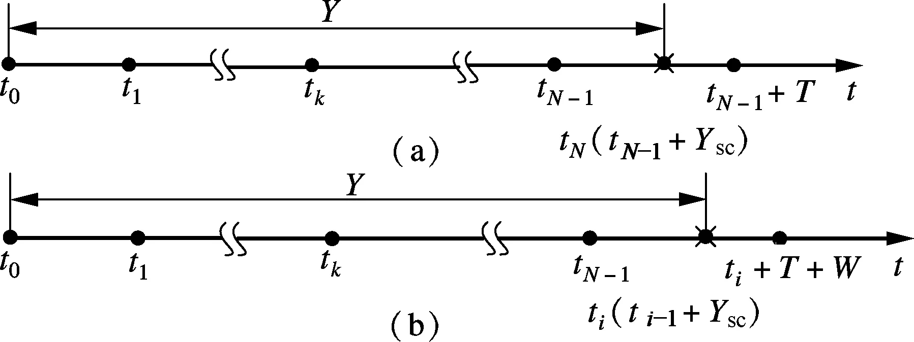
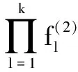
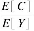
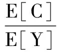
Various approaches have been developed to optimize the PM policy[6]. Most of them ignore the influence of random factors on PM policy, and thus regard that the maintenance period is a fixed value. Actually, it should be a limited random value in practice because of random factors that make the maintenance actions unable to be performed as soon as a planned PM period is reached. Two typical examples of these cases are PM on some Chinese diesel locomotives being 2 300 to 2 600 km[7]and on some Japanese planes for 12 to 18 months[8]. Only a few of them discussed the maintenance optimization for a system with a stochastic PM interval considering a job cycle or a failure occurrence[9-11]. Sheu et al.[9]examined a generalized age replacement policy. In Ref.[9], if a unit fails at agey In the above mentioned research, the maintenance plan is modified by failures or the working cycle of a job, and yet it should be jointly affected by some random external and internal factors in a finite time period in practical. These random factors may result in a modification of the preconcerted PM period in [T-w1,T+w2], whereTis a planned PM period andw1andw2are constant given by engineers. For ease of research, herein setT-w1asTandw1+w2=W. Consequently, the dynamic PM schedule randomly distributes within [T,T+W]. Under this condition, the PM policy is different from the general periodic PM policy, and thus it is termed as a quasi-periodic PM policy in this paper. In our recent study[12], a quasi-periodic replacement policy for a mono-unit system considering the modifications of replacement plans is discussed. By comparison, the quasi-periodic PM for a two-unit series system is widely used in most real cases, although its optimization is more complex. Based on these considerations, an optimal quasi-periodic PM policy for the two-unit series system is introduced in this paper. For a quasi-periodic PM policy, a scheduled PM plan and a dynamic PM plan are presented. The scheduled PM plan is a long-term plan and is predetermined without considering the provisional effects of some random factors. According to the schedule plan, the system is preventively maintained atkT(k=1,2,…,N-1) and replaced atNT. Nevertheless, the dynamic PM plan is a short-term plan considering the effect of some provisional external factors, in which the first (N-1) PM interval is divided into a planned PM period and an implementation period. The length of the planned PM period is a fixed value and made by the scheduled PM plan, while the length of the implementation period is given by engineers’ experience considering some practical needs. The quasi-periodic PM policy for a series system comprised of two units (denoted asU1andU2) is considered. The lifetimes ofU1andU2are random variables (marked asζ1andζ2) with distribution functionF(i)(t) (i=1,2), respectively, and it is assumed thatζ1is stochastically smaller thanζ2.U1is assumed to be repairable and it undergoes minimal repair at failures. Thus,U1failures occur according to a non-homogeneous Poisson process with intensity rateh(1)(t). (1) A replacement of the system contains two cases: planned and unplanned activities. The former occurs when there are no catastrophic failures in each PM interval and when the PM number reaches the thresholdNdetermined by the PM plan. The replacement cycle is shown in Fig.1, where the first (N-1)-th PM actions are executed at the timeti(i=1,2,…,N-1) following dynamic PM plans, and a planned replacement is performed attN(tN-tN-1=T, orYs,N>T). Fig.1 Planned replacement The later is trigged by a catastrophic failure ofU2. The replacement cycle is shown in Fig.2, where the first (i-1)-th PM actions are executed at the timeti-1(i=1,2,…,N) according to the dynamic PM plans (0 Although there are some random factors affecting the PM activities, they may be forecasted in a relative short implementation period in practice. Thus, the system can be completely arranged to be preventively maintained during each implementation period. According to this fact,we assume that the occurring time of a dynamic PM plan,Ysc, is a random variable and follows the uniform distribution with a probability density function 1/Win each implementation period. Fig.2 Unplanned replacement According to the above maintenance description, three model assumptions are given as below: 1) Failures ofU1andU2are independent. All failures can be instantly detected and repaired. 2) The hazard rate function ofU1andU2are continuous, positive, concave and non-decreasing int. After a replacement, the system can be restored to “as good as new” state. 3) All minimal repair, PM, and replacement time are negligible. A replacement cycle is defined as a time interval between an installation of the system and the first replacement or between two consecutive replacements. LetYandCdenote the length of a renewal cycle and the operational cost over a replacement cycle, respectively. Thus, {Y,C} constitutes a renewal reward process. IfC(t) denotes the operational cost over the time interval [0,t), then we have (2) whereE[C] andE[Y] denote thes-expected maintenance cost and thes-expected renewal cycle, respectively. An unplanned replacement may occur in each PM period or ahead of the dynamic PMs in each implementation period ifys,i (3) wherexjis the length of thej-th PM interval;IB(Z) is an indicator function of setB, i.e., (4) Letf(i)(t) denote the pdf ofUi(i=1,2) failures. Furthermore, according to Eqs.(3) and (4), the expected renewal cycle and the maintenance cost can be described as (5) pj(aj-1(T)xj+H(2)(xj))+Cp)+KH(1)(T)+pN(aN-1(T)T+H(2)(T))+ (6) Submitting Eqs.(5) and (6) into Eq.(2), we can obtain the long-run cost rate functiong(T,N). In general, in order to obtain a unique solutionT*andN*by minimizing Eq.(2) with the analytical method, we need to compute the second derivative and the second-order difference ofM(T,N),P(T,N) andS(T,N) with regard toTandNin Eq.(2); however it is difficult to compute them due to their complexity. As a practical application, it is unnecessary to determine a much more precise solution, while a feasible solution is acceptable by a simple method with an allowable deviation. Based on these considerations, the Hooke-Jeeves method is used in this model, which can be applied almost immediately to many nonlinear optimization problems[14]. The detailed steps of the Hooke-Jeeves method can be seen in Ref.[14]. According to the proposed model, there are three special cases with differentWandpi. The brief explanation and the long run expected per unit time are given for each case. 1) WhenW=0,pi≠1, andN>1 In this case, the system is the same as presented in section 1, and the difference between the PM policy and the proposed policy is that the PM period is a fixed valueT. The mean cost rate equation is shown as (7) where 2) WhenW=0,pi=1, andN>1 This model is a special case of the case 1 withpi=1, in which failures ofU2only include minor failures. Periodic PM forU2is mechanical service and forU1is perfect. A replacement is performed when the PM number reaches the thresholdN. The mean cost rate equation is (8) 3) WhenW≠0,pi=1, andN>1 In this case, a quasi-periodic PM policy is executed for one type of the two-unit system. Failures of the system are minor failures. Maintenance service forU2and a perfect PM forU1are stochastically performed in the implementation period. A replacement is performed when the PM number reaches the thresholdN. The mean cost rate equation is described as In this section, the procedures and features of the model are illustrated using the following numerical examples. Eq.(2) is computed in Matlab 2010b using the Hooke-Jeeves algorithms described above. We obtain the optimalT*=1.48,N*=6,Cmin=5.664, andE[Y]=5.648. That is, the PM activities are stochastically performed in the time interval [1.48, 1.78]. The mean cost rateC(N,T) is shown in Fig.3. Fig.3 Three-dimensional plot of (C,T,N) In order to present the sensitivity of the maintenance and failure parameters to the mean cost rate, some numerical examples are given. Tabs.1 and 2 exhibit the change tendency ofT*,N*andCminwith different parametersKp,KrandW. AsW=0.3 and 0.5, the optimal results are shown in Tab.1, respectively. Tab.1 Optimal results with Kp=0.6,r=0.7 From Tab.1 it can be found thatT*,N*andCminobviously increase with the increase ofKrunder a givenKp, whileT*decreases andCminkeeps a slow growth trend with the increase ofWunder a givenKrandKp. The optimalN*has no obvious change with differentWbecause it is mainly determined byCR. Tab.2 shows thatT*,N*andCminalso increase with the increase ofKpunder a givenKr, whileT*andN*decrease andCminincreases slowly with the increase ofWunder a givenKrandKp. Tab.2 Optimal results with Kr=4,r=0.7 In this paper, a quasi-periodic PM policy for one type of two-unit series system considering the influence of some random factors is proposed. Based on our analysis and the examples above, the following conclusions are obtained: 1) The optimalT*andN*can be obtained although the model is complex, and the method used in this paper can also be extended to some special cases proposed above. 2) The increase in the length of the implementation period can cause an increase in the mean cost rate and a decrease in the mean operational time, and thus the choice ofWshould be decreased as soon as possible under the condition of meeting the requirements of practice. 3) The policy proposed in this paper is more convenient for production. It can be replaced by the general PM policy (the special case 3) for a lesserW, while the difference between the proposed policy and the general PM policy should not be ignored ifWis relatively greater. [1]Wu S M.Reliabilityengineering[M]. London: Springer, 2011: 129-140. [2]Nicolai R P, Dekker R. Optimal maintenance of multi-component systems: a review [R]. Rotterdam,Netherlands:Econometric Institute of Erasmus University Rotterdam, 2006. [3]Zhang Y L, Wang G J. A geometric process repair model for a repairable cold standby system with priority in use and repair [J].ReliabilityEngineeringandSystemSafety, 2009,94: 1782-1787. [4]Hanagal D D, Kanade R A. Optimal replacement policies based on number of down times for cold standby system when the lifetime and the repair time are dependent [J].JournalofReliabilityandStatisticalStudies, 2011,4(1): 41-52. [5]Castaniera B, Grallb A, Bérenguerb C. A condition-based maintenance policy with non-periodic inspections for a two-unit series system [J].ReliabilityEngineeringandSystemSafety, 2005,87(1): 109-120. [6]Nicolai R P, Dekker R.Complexsystemmaintenancehandbook[M]. London: Springer, 2008: 263-286. [7]Gao W K, Zhang Z S, Zhou Y F, et al. Optimal combinatorial replacement policy under a given maintenance interval for the combined governor in diesel locomotives [J].EksploatacjaiNiezawodnosc-MaintenanceandReliability, 2013,15(2): 89-98. [8]Kodo I, Toshio N. Optimal operation censoring policy of aircraft [C]//2012Asia-PacificInternationalSymposiumonAdvancedReliabilityandMaintenanceModeling. Nanjing, China, 2012: 184-191. [9]Sheu S H, Kuo C M, Nagagawa T. Extended optimal age replacement policy with minimal repair [J].RAIRO:RechercheOperationnelle, 1993,27(3): 337-351. [10]Castro I T, Sanjuan E L. An optimal maintenance policy for repairable systems with delayed repairs [J].OperationsResearchLetters, 2008,36(5): 561-564. [11]Chen M. Optimal random replacement models with continuously processing jobs [J].AppliedStochasticModelsinBusinessandIndustry, 2012,29(2): 389-398. [12] Gao W K, Zhang Z S, Zhou Y F,et al. Maintenance optimization for a system with an implemented range of replacement activities [C]//2013InternationalConferenceonQuality,Reliability,Risk,Maintenance,andSafetyEngineering. Chengdu, China,2013: 394-398. [13]Tsai Y T, Wang K S, Tsai L C. A study of availability-centered preventive maintenance for multi-component systems [J].ReliabilityEngineeringandSystemSafety, 2004,84(3): 261-270. [14]Lewis R M, Torczon V, Trosset M W. Direct search methods: then and now [J].JournalofComputationalandAppliedMathematics, 2000,124(12): 191-207.1 Model Description


2 Maintenance Optimization


3 Special Cases


4 Numerical Example



5 Conclusion
 Journal of Southeast University(English Edition)2013年4期
