Seasonal and interannual variabilities of mean velocity of Kuroshio based on satellite data

Jun-cheng ZUO, Min ZHANG*, Qing XU, Lin MU, Juan LI, Mei-xiang CHEN

1. Key Laboratory of Coastal Disaster and Defence of Ministry of Education, Hohai University, Nanjing 210098, P. R. China

2. College of Harbor, Coastal and Offshore Engineering, Hohai University, Nanjing 210098, P. R. China

3. South China Sea Prediction Center, South China Sea Branch, State Oceanic Administration, Guangzhou 510310, P. R. China

4. National Marine Data and Information Service, Tianjin 300171, P. R. China

Seasonal and interannual variabilities of mean velocity of Kuroshio based on satellite data

Jun-cheng ZUO1,2, Min ZHANG*3, Qing XU1,2, Lin MU4, Juan LI1,2, Mei-xiang CHEN1,2

1. Key Laboratory of Coastal Disaster and Defence of Ministry of Education, Hohai University, Nanjing 210098, P. R. China

2. College of Harbor, Coastal and Offshore Engineering, Hohai University, Nanjing 210098, P. R. China

3. South China Sea Prediction Center, South China Sea Branch, State Oceanic Administration, Guangzhou 510310, P. R. China

4. National Marine Data and Information Service, Tianjin 300171, P. R. China

Combining sea level anomalies with the mean dynamic topography derived from the geoid of the EGM08 global gravity field model and the CLS01 mean sea surface height, this study examined the characteristics of global geostrophic surface currents and the seasonal and interannual variabilities of the mean velocity of the Kuroshio (the Kuroshio source and Kuroshio extension). The patterns of global geostrophic surface currents we derived and the actual ocean circulation are basically the same. The mean velocity of the Kuroshio source is high in winter and low in fall, and its seasonal variability accounts for 18% of its total change. The mean velocity of the Kuroshio extension is high in summer and low in winter, and its seasonal variability accounts for 25% of its total change. The interannual variabilities of the mean velocity of the Kuroshio source and Kuroshio extension are significant. The mean velocity of the Kuroshio source and ENSO index are inversely correlated. However, the relationship between the mean velocity of the Kuroshio extension and the ENSO index is not clear. Overall, the velocity of the Kuroshio increases when La Niña occurs and decreases when El Niño occurs.

seasonal and interannual variabilities; global gravity field; global geostrophic surface current; mean dynamic topography; Kuroshio

1 Introduction

Ocean circulation and its dynamic characteristics are the basic contents of oceanographic research. They are also significant for understanding and estimating the trend of variations in the climate system.

Outside of the equatorial region, ocean currents over a long time scale (usually more than a few days) are close to the state of the geostrophic balance, and their movement follows therules of geostrophic approximation and hydrostatic balance. As the sea surface topography is directly related to geostrophic surface currents, we can calculate ocean currents through the geostrophic balance equation based on the sea surface topography. The sea surface topography is usually obtained by analysis, assimilation, and calculation of the hydrological data (temperature, salinity, and pressure measured with the expendable bathythermograph (XBT); conductivity, temperature, and depth (CTD) sensors; buoys, etc.). Satellite altimeter observation is another way to obtain the sea surface topography for simulating ocean currents, which began in the 1980s. Although high-precision and high-resolution satellite altimetry data allow for the determination of the fine structure of the mean sea surface height within a wide range at a high speed, the accuracy is not satisfactory in revealing the characteristics of ocean currents, because their dynamic fluctuations require a high independent and definite geoid of the equipotential surface of the global gravity field. Therefore, obtaining an accurate geoid is the key to simulating ocean circulation. After the implementation of the satellite gravity technology, with the advent of models from the new dedicated satellite gravity missions CHAMP (community HIV/AIDS mobilization project) and GRACE (gravity recovery and climate experiment), an independent and high-quality geoid can be determined to form the sea surface topography combined with the sea surface height, and further to obtain a more accurate result of ocean circulation. Tapley et al. (2003), Dobslaw et al. (2004), and Zhou et al. (2008) studied ocean circulation based on the satellite gravity data, and their conclusions were close to the observation result. Alexandre and Joseph (2012) also computed geostrophic surface currents of the South Atlantic Ocean using geoid models, showing that it is an accurate way to research ocean circulation using high-precision satellite data.

We obtained the mean dynamic topography (MDT) by subtracting the geoid of the EGM08 global gravity field model from the CLS01 mean sea surface height (MSSH). Then the absolute dynamic topography (ADT) was computed by combining MDT with dynamic topography anomalies, which are called sea level anomalies (SLA) (Lázaro et al. 2005). We derived global geostrophic surface currents based on the geostrophic balance equation and analyzed their characteristics and the seasonal and interannual variabilities of the mean velocities of the Kuroshio source and Kuroshio extension, providing a foundation for clarifying Kuroshio’s effect on the national and coastal marine environment and investigating its relationship with abnormal climate change and other important issues.

2 Data

2.1 Satellite altimetry data

We used altimetry data from the SSALTO/DUACS multi-satellite (JASON-1, TOPEX/ POSEIDON, ENVISAT, GFO, ERS-1/2, and GEOSAT) integrated data from the National Centre for Space Studies of France, and for this study chose SLA, whose data coverage wasoceanwide between 82ºS and 81ºN with 1/3º Mercator grids. The time sampling interval was seven days, and the time period was from January 1993 to December 2008. The Hamming window filter was adopted for spatial filtering and interpolation. The cut-off radius was 200 km, and the size of the grid interpolation was 0.5° × 0.5°.

2.2 WOA05 temperature and salinity data

WOA05 temperature and salinity data from the U.S. National Oceanographic Data Center are three-dimensional average temperature and salinity fields obtained based on field observations of about seven million ocean temperature profiles. They contain annual average, seasonal average, and monthly average data obtained on the basis of objective analysis of the world ocean database of the year 2001. There are 33 vertical standard layers (from 0 to 5 500 m under the sea surface) for annual and seasonal average data and 24 layers (from 0 to 1 500 m under the sea surface) for monthly average data. We chose the annual average data, with a coverage region oceanwide between 89.5ºS and 89.5ºN and a horizontal resolution of 1º × 1º, to calculate ocean circulation. The calculated results were compared with geostrophic surface currents obtained from the satellite data.

2.3 Datasets of MSSH and geoid used for obtaining MDT

The CLS01 MSSH we used was developed by the CLS Space Oceanography Division of France. MSSH of high quality was computed using a seven-year TOPEX/POSEIDON mean profile, a five-year ERS-1/2 mean profile, a two-year GEOSAT mean profile, and two series of 168-day non-repeating cycle data of the ERS-1 geodetic phase. The coverage region of the data was oceanwide between 80ºS and 82ºN, and the grid resolution was 1/30º. The EGM08 global gravity field model developed by the U.S. National Geospatial-Intelligence Agency (NGA) EGM Development Team was also used. This gravitational model was further developed with the improved versions of 5′ × 5′ global gravity databases and GRACE-derived satellite solutions. It is complete to spherical harmonic degree and order 2159 with a geoid accuracy of 15 cm (RMS) worldwide. The key to the success of this endeavor is the compilation of a complete and accurate 5′ × 5′ global gravity anomaly database that takes advantage of all the latest data and is capable of modeling both land and marine areas worldwide. The coverage region of the data was oceanwide between 90ºS and 90ºN. The CLS01 MSSH and geoid of EGM08 global gravity field model are both related to the same conventional ellipsoid of revolution. MDT was derived by subtracting the geoid of the EGM08 global gravity field model from CLS01 MSSH, with the Hamming window filter used for spatial filtering and interpolation. The cut-off radius was 200 km. The coverage region of the MDT data was oceanwide between 80°S and 82°N with a grid size of 0.5° × 0.5° (Fig. 1).

3 Results and discussion

3.1 Global geostrophic surface currents

We calculated global geostrophic surface currents (Fig. 2) with MDT based on the following geostrophic balance equations (Eqs. (1) and (2)) (Knudsen 1993) for an oceanwide region between 66°S and 66°N. The geostrophic surface current near the equatorial region (0.75°S to 0.75°N) was not calculated.

where u and v are the velocity components of global geostrophic surface currents in the eastward and northward directions, respectively; ξis the mean dynamic topography; ϕ and λ are the latitude and longitude, respectively; f is the Coriolis parameter, and f = 2ωesin ϕ, where ωeis the earth’s angular velocity; g is the gravitational acceleration; and R is the earth’s mean radius.

From Fig. 2, it can be seen clearly that a clockwise circulation forms in the North Pacific Ocean, caused by the main stream system, which consists of the North Equatorial Current, the Kuroshio, the North Pacific Current, and the California Stream. The South Equatorial Current, the Equatorial Countercurrent, the Alaska Stream, and the Oyashio can also be seen clearly. The equatorial current in the Indian Ocean and Atlantic Ocean, the Gulf Stream in the Atlantic Ocean, and the Antarctic Circumpolar Current are also evident.

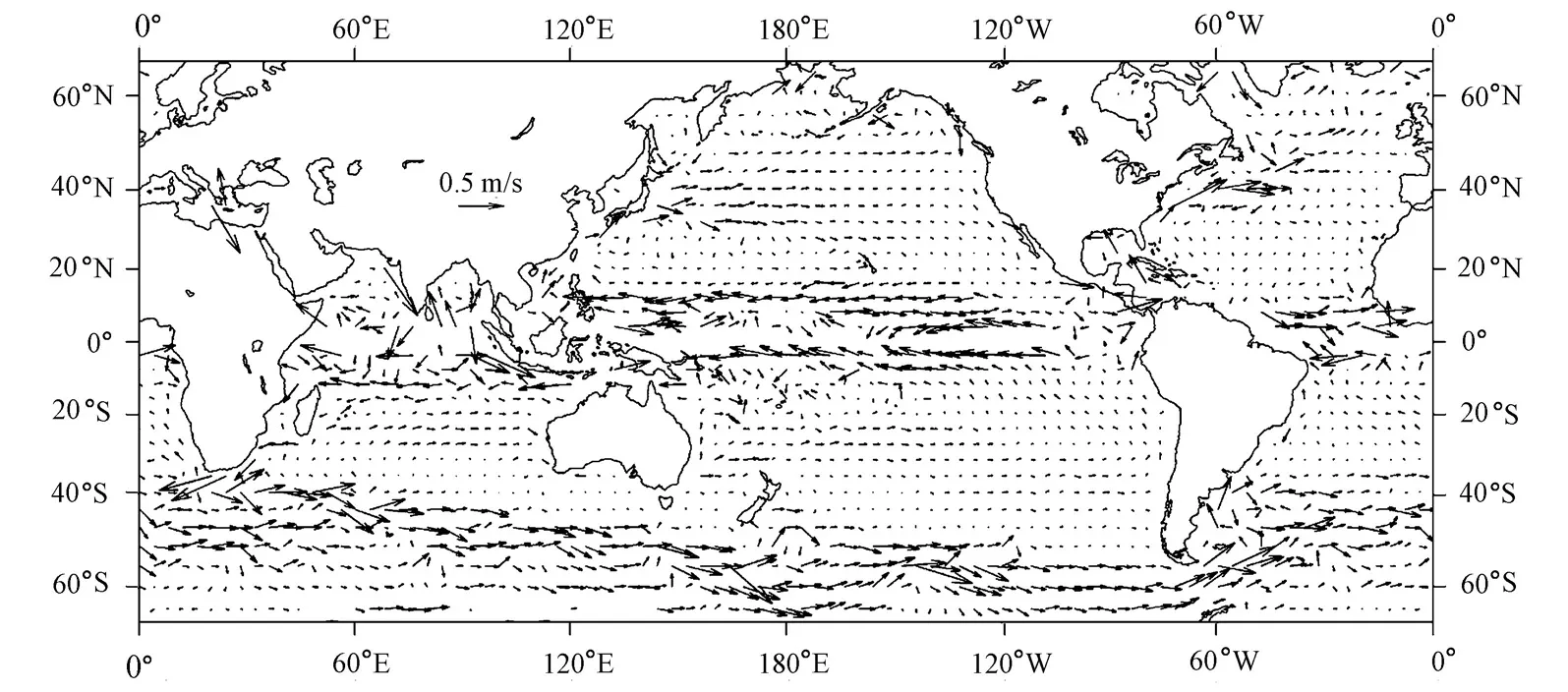
Fig. 2Global geostrophic surface currents calculated with MDT

(1) The North Equatorial Current occurs between 6°N and 18°N and strengthens gradually from the east to the west. It divides into the north and south branches when arriving at the west bank. The north branch forms the famous Kuroshio. When the Kuroshio flows northward through the Luzon Strait, a small part of it flows into the South China Sea, and most of it invades into the East China Sea from the north of the Taiwan Strait and then turns to the northeast, where it further divides into two branches near the northern sea area of the Ryukyu Islands. One branch has a northwest deflection and then turns northeastward into the Sea of Japan through the Tsushima/Korea Strait, and the other branch turns northward along the southern bank of the Japanese islands with a little clockwise deflection. The eastward bypass appears in the 34°N section, and part of it continues to flow northward and meets with the southward Oyashio, flowing together to form the eastward North Pacific Current. The current flows towards the east bank of the Pacific Ocean, then turns southward as it is blocked by the mainland border near California, and finally enters the North Equatorial Current. The maximum velocity of the Kuroshio reaches 0.5 m/s in the region of 27°N to 33°N and 135°E to 138°E.

(2) Near the equator in the Pacific Ocean, the eastward Equatorial Countercurrent and the westward South Equatorial Current form a clockwise circulation system. The Equatorial Countercurrent occurs between 0°N and 6°N with high velocities. The South Equatorial Current occurs between 0°S and 18°S with a wide flow region. The maximum velocities of the North and South Equatorial currents reach 0.4 m/s.

(3) In the Indian Ocean, the South Equatorial Current occurring near the east sea area of Madagascar is also very clear. There is a wide band of zonal South Equatorial Current to the west of Madagascar. The geostrophic surface current in the Agulhas area has a velocity up to 0.3 m/s.

(4) The Gulf Stream is also very clear with the maximum velocity reaching 0.4 m/s.

(5) The Antarctic Circumpolar Current has a significant northward extension in the Atlantic and Indian oceans. When passing through the southern Pacific Ocean, the Antarctic Circumpolar Current depresses southward due to the flow boundary of New Zealand and the Drake Passage. The maximum velocity of the Antarctic Circumpolar Current reaches 0.4 m/s.

In order to compare the global geostrophic surface currents computed with satellite gravity data, we calculated the ocean circulation (Fig. 3) with the WOA05 temperature and salinity data using the Helland-Hansen formula, taking the depth of 1 000 m as the zero-velocity surface (Sun et al. 2008). Global geostrophic surface currents determined by the satellite gravity data and the surface circulation determined by the temperature and salinity data are almost consistent. The velocity magnitudes of the Kuroshio and Gulf Stream are the same. However, the velocity of the Antarctic Circumpolar Current based on thermohaline data in Fig. 3 is relatively smaller than what has been observed, the maximum value of which is just 0.1 m/s. In addition, there is strong turbulence near the equatorial current, which is anamorphic. The Alaska Stream and California Stream are not clear, which may be partly due to the error caused by the selection of the zero-velocity surface. We can find from these two figures that global geostrophic surface currents computed with satellite data (Fig. 2) are more consistent with those of previous observations and can display more details about the surface circulation. Therefore, this is an accurate way of researching global geostrophic surface currents using high-precision satellite data.

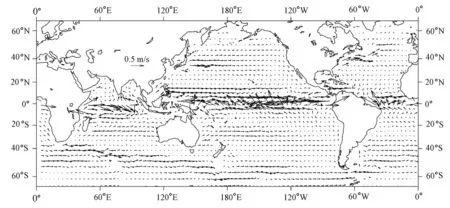
Fig. 3Global surface circulation calculated with WOA05 temperature and salinity data

3.2 Seasonal and interannual variabilities of mean velocity of Kuroshio

We obtained monthly average ADT of 16 years by combining monthly average SLA from January 1993 to December 2008 with MDT. They were taken into the geostrophic balance Eqs. (1) and (2) for simulating the variability of geostrophic surface currents. This paper defines the northward direction as the main direction of the velocity of the Kuroshio source, and the eastward direction as the main direction of the velocity of the Kuroshio extension. We averaged the velocity in the main direction of the Kuroshio to describe the flow intensity of the Kuroshio. The mean velocity is defined as

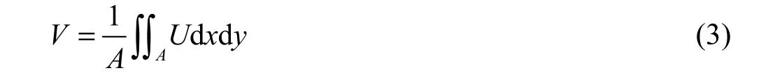
where V is the mean velocity, A is the area where the Kuroshio occurs, and U is the velocity in the main direction of the Kuroshio. The mean velocity is an average value over a certain region. 3.2.1 Seasonal and interannual variabilities of mean velocity of Kuroshio source

Within the region of 15°N to 22°N and 120°E to 130°E of the Kuroshio source, Cai et al.(2009) selected the region of 120°E to 130°E at the 18°N section to study the flux variability of the Kuroshio source. Based on their research, we defined the flow with its northward component of velocity being larger than 20 cm/s as the Kuroshio. We obtained the monthly mean velocity of the Kuroshio source from 1993 to 2008 (Fig. 4).

After making the power spectrum analysis for the mean velocity, we could find cycles of five to eight months, 11 to 12 months, and 32 months which are similar to the ENSO cycles. Using the stochastic dynamic prediction method, we obtained the amplitudes of the annual signal, semi-annual signal, and 28-month signal of the mean velocity of the Kuroshio source which are 0.2 cm/s, 0.5 cm/s, and 0.5 cm/s, respectively. It can be seen in Fig. 4 that the total changing range of the monthly mean velocity of the Kuroshio source is about 8 cm/s, so its seasonal variability accounts for 18%. The seasonal change (semi-annual cycle change) and ENSO-based interannual change account for the majority of the mean velocity variability of the Kuroshio source.

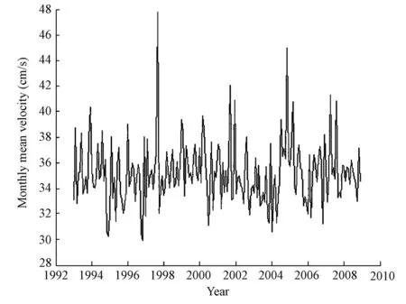
Fig. 4Monthly mean velocity of Kuroshio source

We divided the year into four boreal seasons: January to March as winter, April to June as spring, July to September as summer, and October to December as fall (Lázaro et al. 2005). The changing processes of annual, semi-annual, and 28-month signals of the mean velocity are shown in Fig. 5 and Fig. 6. In the annual signal, the mean velocity of the Kuroshio source reaches the maximum value in June (spring) and minimum in December (fall) every year. In the semi-annual signal, the maximum mean velocity is in February (winter) and August (summer), and the minimum mean velocity is in May (spring) and November (fall). By superposition of the annual signal and semi-annual signal, we can determine that the mean velocity of the Kuroshio source is high in winter and low in fall. This conclusion is the same as that of Wyrtki (1961).

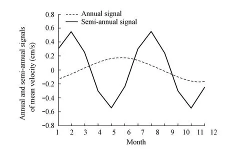
Fig. 5Annual and semi-annual signals of mean velocity of Kuroshio source

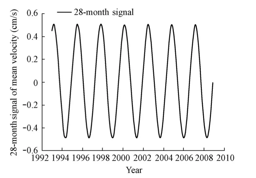
Fig. 6 28-month signal of mean velocity of Kuroshio source

In order to analyze the interannual variability of the mean velocity of the Kuroshio source, we centralized the time series of the mean velocity and removed the trends and signals of annual and semi-annual cycles. As the residual series still contained a lot of high-frequency signals, we processed the residual series and the ENSO index with a one-year low pass filter. From Fig. (7), we can find that the mean velocity of the Kuroshio source is almost inversely varied with the ENSO index. The ENSO index had negative phases in 1996 and 1998 to 1999 when La Niña occurred. It can be concluded that the mean velocity of the Kuroshio source increases when La Niña occurs. In the El Niño years of 1997 and 1998, the mean velocity decreased, and this result can also be found in Cai et al. (2009). Chen (2009) also pointed out that the North Equatorial Current weakens in El Niño years and strengthens in La Niña years. The Kuroshio originates from the north branch of the North Equatorial Current, and the interannual variability of flow of the Kuroshio source is almost the same as that of the North Equatorial Current.

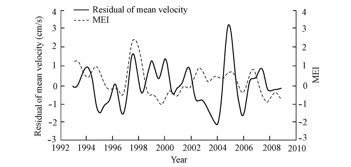
Fig. 7Residual series of mean velocity of Kuroshio source and multivariate ENSO index (MEI) processed with one-year low pass filter

3.2.2 Seasonal and interannual variabilities of mean velocity of Kuroshio extension

We selected the region from 25°N to 45°N and 135°E to 180°E for studying the Kuroshio extension. According to Polovina et al. (2006), we defined the flow with its eastward component of velocity being larger than 20 cm/s as the Kuroshio. We obtained the monthly mean velocity of the Kuroshio extension from 1993 to 2008 (Fig. 8).

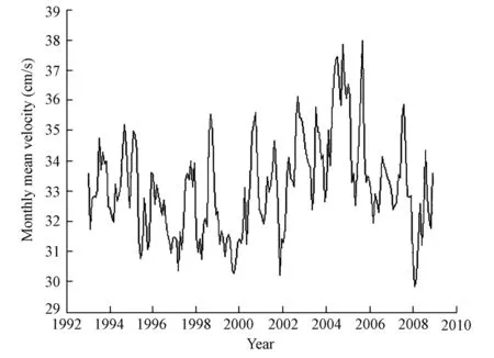
Fig. 8Monthly mean velocity of Kuroshio extension

Conducting the power spectrum analysis for the mean velocity of the Kuroshio extension, we can find relatively significant periods of mean velocity of six to eight months in addition to the annual cycle, showing obvious seasonal and interannual variabilities of the velocity of the Kuroshio extension. We extracted signals of annual, semi-annual, and 28-month cycles (Figs. 9 and 10), and their change amplitudes are 0.7 cm/s, 0.3 cm/s, and 0.5 cm/s, respectively. The signal of the annual cycle shows that the maximum mean velocity occurs in September (summer), and the minimum mean velocity occurs in March (winter). In the semi-annual signal, the maximum mean velocity occurs in February and August, and the minimum mean velocity occurs in May and November. The annual cycle of the mean velocity is the main pattern of seasonal variability. Overall, the mean velocity of the Kuroshio extension is high in summer and low in winter. This result is the same as that of Sekine and Kutsuwada (1994). Fig. 8 shows that the total changing range of the mean velocity of the Kuroshio extension is about 8 cm/s, and that the seasonal variability accounts for 25%.

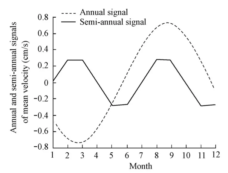
Fig. 9Annual and semi-annual signals of mean velocity of Kuroshio extension

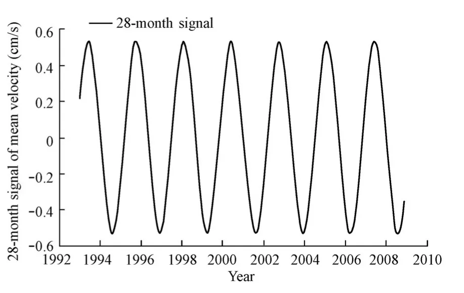
Fig. 1028-month signal of mean velocity of Kuroshio extension

The interannual variability of the mean velocity of the Kuroshio extension is significant. We centralized the time series of the mean velocity and removed the trends and signals of annual and semi-annual cycles in order to study its interannual variability. The residual series and the ENSO index were processed with a one-year low pass filter (Fig. 11). The correlation of the mean velocity of the Kuroshio extension with the ENSO index is not significant, butthere are some connections. We found that the mean velocity decreased after the summer of 1997 when El Niño occurred, and then increased after June 1998 when La Niña occurred.

Fig. 11Residual series of mean velocity of Kuroshio extension and MEI processed with one-year low pass filter

3.3 Annual mean velocity of Kuroshio

We calculated the annual mean velocities of the Kuroshio source and Kuroshio extension (Fig. 12). The two velocity series are negatively correlated, with a maximum correlation coefficient of –0.799, showing that there is a definite link between the interannual variabilities of the two data series. However, the correlation coefficient between the two monthly mean velocity series is only 0.06, because the Kuroshio source originates from the north branch of the North Equatorial Current but the Kuroshio extension is impacted by the local ocean-atmosphere and dynamic factors in the East China Sea.

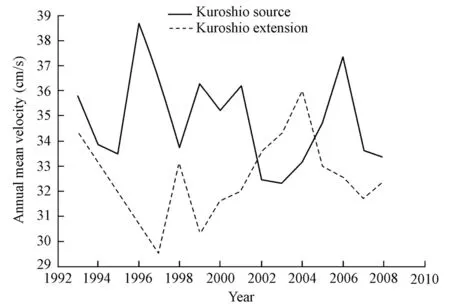
Fig. 12Annual mean velocity of Kuroshio source and Kuroshio extension

4 Conclusions

The MDT was derived based on the satellite gravity and satellite altimetry data, and then global geostrophic surface currents were computed with the geostrophic balance equation and compared with the surface circulation calculated with the temperature and salinity data. The obtained MDT can reveal characteristics of geostrophic surface currents well. Combining the monthly sea level anomaly data of nearly 16 years with the MDT, we investigated the seasonaland interannual variabilities of the mean velocities of the Kuroshio source and Kuroshio extension, and obtained the following conclusions:

(1) The monthly mean velocity of the Kuroshio source has significant seasonal variability. The mean velocity is high in winter and low in fall. The amplitude of the mean velocity is 0.2 cm/s for the annual cycle and 0.5 cm/s for the semi-annual cycle. The seasonal change accounts for 18% of the total change. Interannual variability of the mean velocity of the Kuroshio source is also significant, and the mean velocity almost inversely varies with the ENSO index. The mean velocity decreases when El Niño occurs and increases when La Niña occurs.

(2) The amplitude of the mean velocity is 0.7 cm/s for the annual cycle and 0.3 cm/s for the semi-annual cycle of the Kuroshio extension. The mean velocity of the Kuroshio extension is high in summer and low in winter. The seasonal change accounts for 25% of the total change. The correlation between the mean velocity of the Kuroshio extension and the ENSO index is not obvious, but there are some connections. El Niño phenomenon weakens the mean velocity of the Kuroshio extension, and the La Niña phenomenon enhances it.

(3) The maximum correlation coefficient between the annual mean velocities of the Kuroshio source and Kuroshio extension reaches –0.799, showing that there is a definite link between the interannual variabilities of the two data series. However, the correlation coefficient between the monthly mean velocities of the Kuroshio source and Kuroshio extension is only 0.06, because the Kuroshio source is a branch of the North Equatorial Current but the Kuroshio extension is impacted by the local ocean-atmosphere and dynamic factors in the East China Sea.

(4) The consistency of the present results about global geostrophic surface currents and the seasonal and interannual variabilities of the mean velocities of the Kuroshio source and Kuroshio extension with those of previous studies shows that this is an effective way to study the ocean circulation using high-precision satellite data. For the coastal zone, there are still some differences between the calculated geostrophic surface currents and the actual currents due to the limitation of the precision of the satellite gravity data. Considering the fact that the satellite gravity data are not accurate enough for small-scale signals, we filtered the small-scale circulation signals, and only studied the large-scale circulation features. The implementation of the gravity satellite program of the Gravity Field and Steady-State Ocean Circulation Explorer may greatly enhance the accuracy and spatial resolution of the global gravity field, which is of great significance to the description of medium-scale and small-scale surface circulations (Pail et al. 2010; Knudsen et al. 2011).

Alexandre, B. L., and Joseph, H. 2012. Use of recent geoid models to estimate mean dynamic topography and geostrophic currents in south Atlantic and brazil Malvinas confluence. Brazilian Journal of Oceanography, 60(1), 41-48. [doi:10.1590/S1679-8759201200010000]

Cai, R. S., Zhang, Q. L., and Qi, Q. H. 2009. Characters of transport variations at the source and adjacent area of Kuroshio. Journal of Oceanography in Taiwan Strait, 28(3), 299-306. (in Chinese)

Chen, M. X. 2009. Dynamics of Sea Level Variation in the North Pacific Ocean, Kuroshio Region of East Sea of China and Kuroshio Extension. Ph. D. Dissertation. Qingdao: Ocean University of China. (in Chinese)

Dobslaw, H., Schwintzer, P., Barthelmes, F., Flechtner, F., Reigber, C., Schmidt, R., Schöne, T., and Wiehl, M. 2004. Geostrophic Ocean Surface Velocities from TOPEX Altimetry, and CHAMP and GRACE Satellite Gravity Models, 1-22. Potsdam: Geoforschungszentrum Potsdam.

Knudsen, P. 1993. Integration of gravity and altimeter data by optimal estimation techniques. Satellite Altimetry in Geodesy and Oceanography, 50, 453-466. [doi:10.1007/BFb0117935]

Knudsen, P., Bingham, R., Andersen, O., and Rio, M. H. 2011. A global mean dynamic topography and ocean circulation estimation using a preliminary GOCE gravity model. Journal of Geodesy, 85(11), 861-879. [doi:10.1007/s00190-011-0485-8]

Lázaro, C., Fernandes, M. J., Santos, A. M. P., and Oliveira, P. 2005. Seasonal and interannual variability of surface circulation in the Cape Verde region from 8 years of merged T/P and ERS-2 altimeter data. Remote Sensing of Environment, 98(1), 45-62. [doi:10.1016/j.rse.2005.06.005]

Pail, R., Goiginger, H., Schuh, W. D., Hock, E., Brockmann, J. M., Fecher, T., Gruber, T., Mayer-Gurr, T., Kusche, J., Jaggi, A., and Rieser, D. 2010. Combined satellite field model GOCO01S derived from GOCE and GRACE. Geophysical Research Letters, 37, L20314. [doi:10.1029/2010GL044906]

Polovina, J., Uchida, I., Balazs, G., Howell, E., Parker, D., and Dutton, P. 2006. The Kuroshio extension bifurcation region: A pelagic hotspot for juvenile loggerhead sea turtles. Deep Sea Research Part II: Topical Studies in Oceanography, 53(3-4), 326-339. [doi:10.1016/j.dsr2.2006.01.006]

Sekine, Y., and Kutsuwada, K. 1994. Seasonal variation in volume transport of the Kuroshio south of Japan. Journal of Physical Oceanography, 24(2), 26l-272. [doi:10.1175/1520-0485(1994)024＜0261:SVIVTO> 2.0.CO;2]

Sun, L., Li, X. B., Yu, J. H., and Wang, S. L. 2008. Analysis of the geostrophic current of Northwest Pacific in ENSO years. Marine Forecasts, 25(3), 86-91. (in Chinese)

Tapley, B. D., Chambers, D. P., Bettadpur, S., and Ries, J. C. 2003. Large scale ocean circulation from the GRACE GGM01 geoid. Geophysical Research Letters, 30(22), 2163-2166. [doi:10.1029/2003GL 018622]

Wyrtki, K. 1961. Physical Oceanography of Marine Investigations of the South China Sea and Gu1f of Thailand, 1959-1961. Ca1ifornia: Scripps of Institution of Oceanography.

Zhou, X. H., Wang, H. B., and Zhan, J. G. 2008. Study on upper layer geostrophic circulation in China marginal sea by use of data of satellite gravity and satellite altimetry. Journal of Geodesy and Geodynamics, 28(4), 83-88. (in Chinese)

(Edited by Ye SHI)

This work was supported by the National Basic Research Program of China (973 Program, Grant No. 2007CB411807), the National Marine Public Welfare Research Project of China (Grants No. 201005019, 201105010-12, and 201105009), and the National Natural Science Foundation of China (Grants No. 40976006 and 41276018-74).

*Corresponding author (e-mail: zhangminling6688@126.com)

Received May 27, 2011; accepted Dec. 28, 2011