Shallow Convection Dataset Simulated by Three Different Large Eddy Models

Yaxin ZHAO, Xiaocong WANG, Yimin LIU, Guoxiong WU, and Yanjie LIU

1College of Earth and Planetary Sciences, University of Chinese Academy of Sciences (UCAS), Beijing 100029, China

2State Key Laboratory of Numerical Modeling for Atmospheric Sciences and Geophysical Fluid Dynamics (LASG),Institute of Atmospheric Physics (IAP), Chinese Academy of Sciences (CAS), Beijing 100029, China

ABSTRACT

Key words: large eddy simulation, SAM, WRF, UCLA-LES, shallow convection, entraining process

1.Introduction

Shallow convection frequently occurs in the trade wind regions.It redistributes energy and water by transporting heat and moisture from the near-surface to higher altitudes,thus affecting the vertical structure of thermodynamic fields.By moistening the middle and lower troposphere, shallow convection facilitates the triggering of deep convection(Neggers et al., 2007; Stevens, 2007; Schiro et al., 2016;Schiro and Neelin, 2019), which is important in the propagation of convectively coupled equatorial waves and disturbances (Ling et al., 2013; Wang and Zhang, 2014).Moreover, shallow convective clouds in the subtropics cool the Earth by increasing the reflection of the incoming solar radiation, thus greatly influencing climate change as well (Bony and Dufresne, 2005; Miao et al., 2021).Therefore, shallow convection must be adequately represented in large-scale models, yet its parameterization remains a great challenge, due to the lack of high-resolution observations (Tiedtke, 1989;Bechtold et al., 1996; Li and Zhang, 2016).

In the last two decades, large eddy models have been widely used for verifying and improving the parameterization of shallow convection (Siebesma et al., 2003; Miao and Jiang, 2004; Wang and Zhang, 2015; Liu et al., 2016; Gu et al., 2020; Wang et al., 2022; Zhu et al., 2023).Large eddy simulation (LES), which typically runs at a horizonal resolution of 100 m, explicitly resolves cumulus scales and acts as a surrogate for real data, providing subgrid-scale(SGS) information that is unavailable from traditional observations.By utilizing LES data, Siebesma and Cuijpers(1995) evaluated assumptions used in the parameterization of shallow cumulus convection and diagnosed bulk entrainment/detrainment rates.This was later followed by De Rooy and Siebesma (2008), who improved the parameterization of entrainment/detrainment rates based on LES results.Besides, Neggers (2009) put forward a dual-mass flux framework for boundary layer convection using LES results.

Since large eddy models are not fine enough to resolve eddies across all scales, they require parameterizations of SGS processes, such as turbulence, which inevitably introduces uncertainties in the LES modeling (Siebesma et al.,2003).In addition, shallow convection occurring over land and ocean should be distinguished, and more shallow convection cases are needed to make the parameterization more universal.In this study, four shallow convection cases with varying inversion strength were simulated by three different large eddy models.

The remainder of the paper is structured as follows:The models and experimental design are introduced in section 2.Section 3 compares the performances of the models with respect to selected variables, including wind, the thermodynamic field, cloud, and SGS variables.Also explored in this section is the model sensitivity to the SGS turbulence scheme.Section 4 provides data records and usage notes.Conclusions are given in section 5.

2.Description of cases and LES models

2.1.Shallow convection cases

Four shallow convection cases are used in this study-namely, Rain in Cumulus over the Ocean (RICO)(Vanzanten et al., 2011), the Barbados Oceanographic and Meteorological Experiment (BOMEX) (Siebesma et al.,2003), the Atlantic Trade Wind Experiment (ATEX)(Stevens et al., 2001), and the Atmospheric Radiation Measurement Program-Southern Great Plains site (ARM-SGP)(Brown et al., 2002).The first three cases are for marine equilibrium trade cumuli that differ in inversion strength, and the last case is for transient continental cumuli, thus spanning a wide range of shallow cumulus regimes.All cases come from the Global Energy and Water Cycle Experiment(GEWEX) Cloud System Studies (GCSS) Working Group on boundary layer clouds, with the locations marked in Fig.1.

Profiles of the large-scale forcing used to drive the LES models are shown in Fig.2, and the surface forcings (i.e., sensible and latent heat flux) are listed in Table 1.For the three maritime cases, subsidence in the lower troposphere dries the atmosphere, which partially offsets the convective moistening.Horizontal advective cooling and drying also serve to counteract the warming and moistening caused by shallow convection, ensuring models quickly reach a steady state.For ARM-SGP, the large-scale forcing varies with time,roughly depicting the life cycle of shallow convection.Other relevant variables, such as surface pressure and temperature, are given in Table 1.

2.2.LES models

The three large eddy models are the System for Atmospheric Modeling (SAM), developed by Khairoutdinov and Randall (2003), UCLA-LES, described in Stevens (2005),and the large-eddy model of the Weather Research and Forecasting model (WRF) (Yamaguchi and Feingold, 2012).All these models solve prognostic equations for the three components of velocity (u, v, w) and the variables specifying the thermodynamic state.The dynamical frameworks of SAM and UCLA-LES are based on the anelastic equations of motion in height coordinates, while WRF uses fully compressible equations in terrain-following hydrostatic-pressure vertical coordinates.Besides, the models differ in the way they parametrize the SGS fluxes.While SAM and WRF use 1.5-order SGS closure based on prognostic SGS turbulent kinetic energy (TKE), UCLA-LES uses Smagorinsky-type closure instead.For non-precipitating shallow convection cases in this study, the precipitation process is turned off to make sure total water is exactly conserved during model integration.Therefore, differences due to cloud microphysics are excluded.

Fig.1.Location map of four shallow convection cases: RICO (red), BOMEX (orange), ATEX (green)and RICO (purple).

All LES models are configured as follows: For BOMEX and ATEX, the models use a horizontal resolution of 64 × 64, with a grid spacing of 100 m and a vertical resolution of 75 levels from the ground to 3000 m.For ARM-SGP and RICO, the horizontal domain is expanded to 128 × 128 and the vertical layers increased to 100 levels, with the horizonal and vertical resolution remaining unchanged.While SAM and UCLA-LES use a constant resolution of 40 m in altitudinal coordinates, WRF uses terrain-following hydrostatic-pressure vertical coordinates that are unequally spaced in the vertical direction.All models are integrated for 6 h for BOMEX, 8 h for ATEX, 14 h for ARM-SGP,and 24 h for RICO.Details of these experimental designs are documented in Siebesma et al.(2003) for BOMEX, Vanzanten et al.(2011) for RICO, Stevens et al.(2001) for ATEX, and Brown et al.(2002) for ARM-SGP.

3.Model performance

3.1.Horizontal winds and thermodynamic fields

Figure 3 shows the initial (grey lines) and the last 4-h mean profiles of domain-averaged potential temperature(θ)and total water (qt).For each case, the model simulations generally bear close resemblance to each other, although differences exist in the simulatedqtwithin the boundary layer.Compared to SAM and UCLA-LES, WRF appears to be more efficient in transporting moisture to upper levels, making the free troposphere wetter and the boundary layer drier.Such a phenomenon is, however, not observed in ARM-SGP.

Figure 4 shows the mean profiles of horizontal winds for the last 4 h, along with the initial one.Also superimposed is the multi-model mean (MMM; black line) and the width of twice the standard deviation of the results of all LES models(gray shading).The geostrophic wind is set to the same as the initial, which decreases with increasing height.Due to the Coriolis force, all models produce an increase in the meridional wind speed and a decrease in the zonal wind speed.The differences among the models are relatively larger than those seen in temperature and humidity.

3.2.Clouds and SGS variables

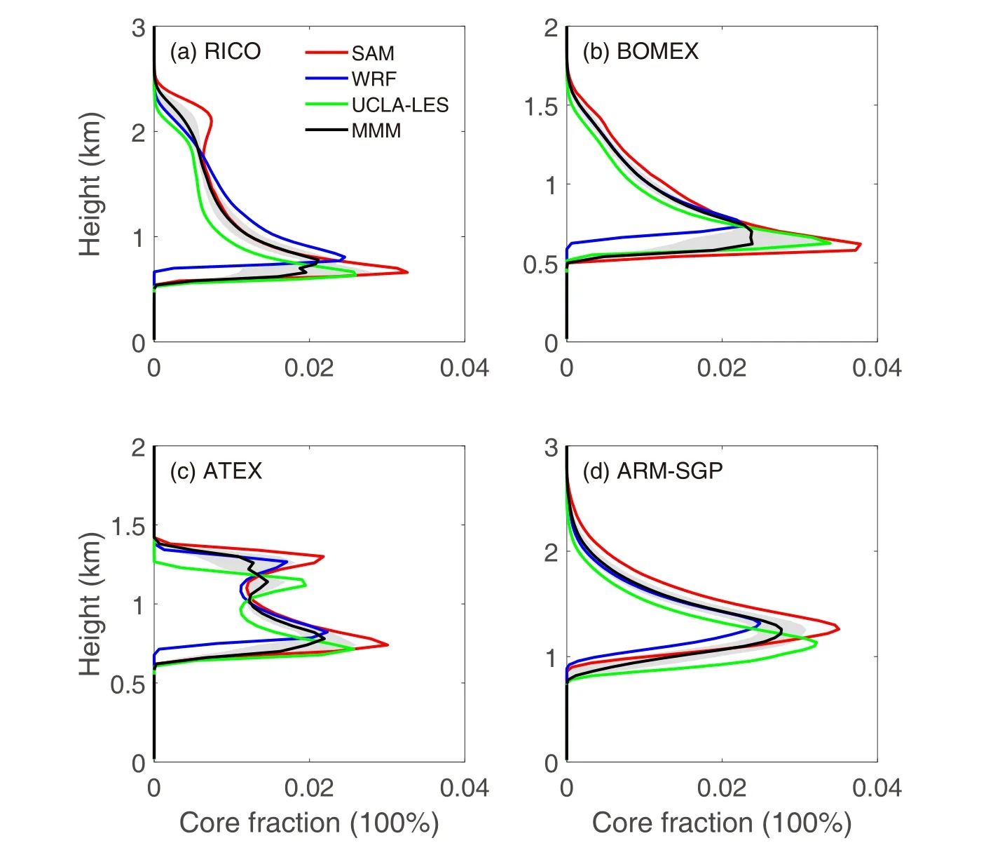
This subsection evaluates the simulation of clouds and SGS variables.Figure 5 shows the mean profiles of the convective core fraction for the four cases, in which red, blue,green, and black lines denote results from SAM, WRF,UCLA-LES, and the MMM, respectively.The convective core here refers to the rising plumes that experience positive buoyancy and contain condensed liquid water, which is important for convective eddy transport (Siebesma and Cuijpers,1995).The core fraction has a maximum near the cloud base, and decreases with increasing height, except for ATEX where a secondary peak forms near the cloud top due to strong inversion.All three models show similar profiles in each case.Overall, the WRF model tends to produce a higher cloud base and smaller core fraction compared with the other two models.The difference in cloud base height between WRF and the other two models is partly due to the different vertical coordinates used by the different models.

Fig.2.Large-scale forcing of (a-d) temperature, (e-h) moisture, and (i-l) vertical velocity (w).From top to bottom are for RICO, BOMEX, ATEX and ARM-SGP.In ARM-SGP, the grey, deep grey, and black lines represent largescale forcings at the 1130, 1430 and 1730 LST (LST= UTC-6), respectively.

As mentioned previously, the main role of shallow convection is to redistribute heat and moisture in the vertical direction.For any conserved variable ϕ, the SGS flux can be decomposed into three terms:

where an overbar stands for the average, a prime represents deviation from the mean value within the plume, α is the convective cloud fraction, and the superscripts c and e stand for the active cloudy part and the surrounding environment,respectively.A widely used assumption in cumulus convection parameterization is that in-cloud and environmental turbulence are much smaller than the organized turbulence term[third term on the right-hand side of Eq.(1)], which describes the contribution due to mean organized updrafts and compensating subsidence in the ambient environment,and thus the first two terms on the right-hand side of Eq.(1)can be dropped, also known as the top-hat approximation(Wang and Stevens, 2000).To verify the plausibility of tophat approximation, the organized turbulent flux (dashed lines) and the full SGS flux (solid lines) of total water are shown in Fig.6.Indeed, the organized turbulent flux is close to the full SGS flux within the convective layers.The models show similar profiles but different magnitudes for the organized turbulent fluxes.Compared to WRF and UCLA-LES, SAM produces larger fluxes because of greater simulation of the core fraction (Fig.5).

Fig.4.Initial (pink) and the last 4-h mean profiles of domainaveraged zonal ( U, solid line) and meridional wind ( V, dashed line) simulated by SAM (red), WRF (blue), and UCLA-LES(green), for the cases of (a) RICO, (b) BOMEX, (c) ATEX, and(d) the temporal mean profiles between 1130 and 1530 LST for ARM-SGP.The black line denotes the MMM, and the gray shading denotes the width of twice the standard deviation of the results of all LES models.

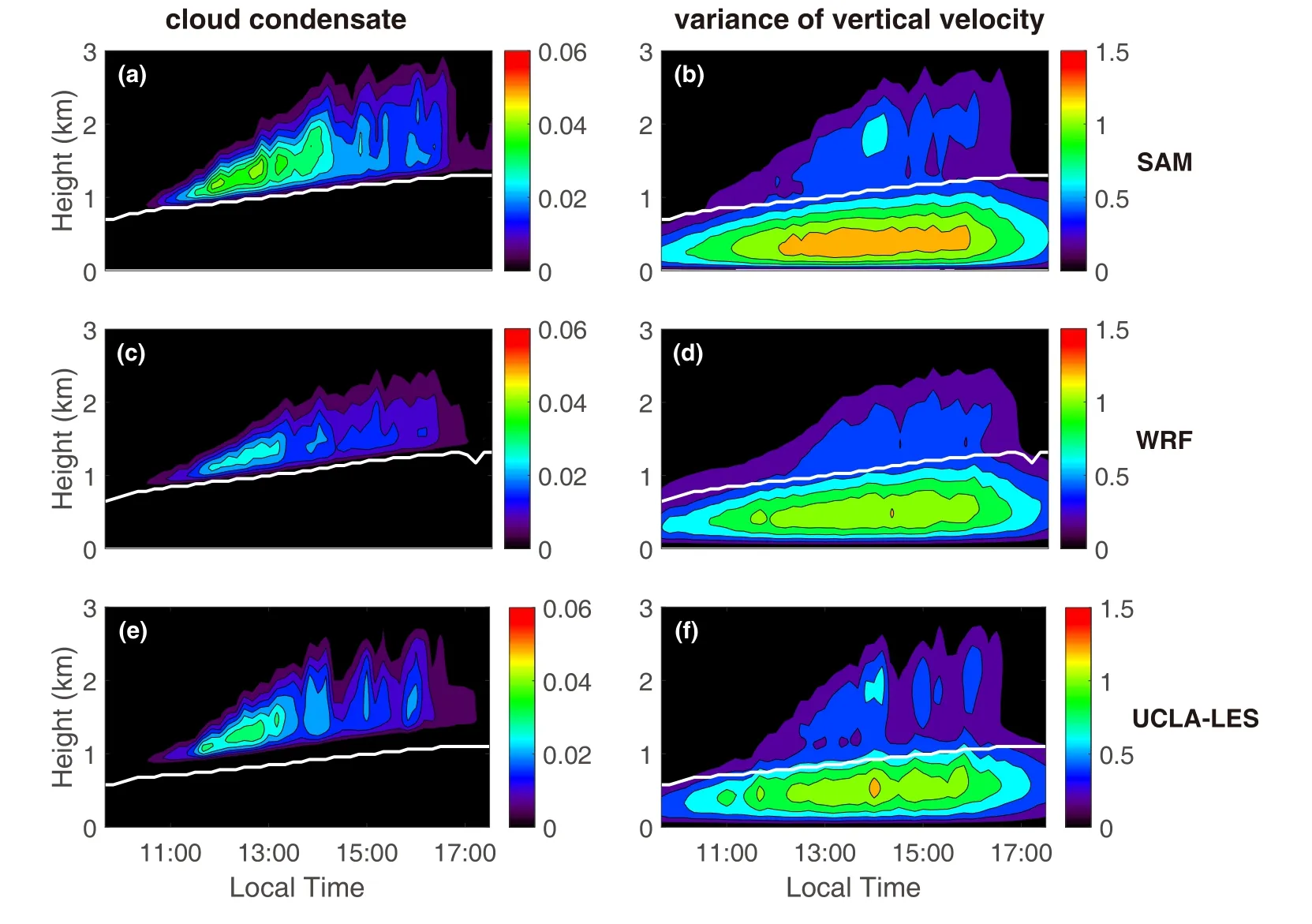
The ARM-SGP case targets the evolution of the convective boundary layer (CBL).Figure 7 shows the temporal evolution of the mean profiles of cloud condensate (left) and variance of the vertical velocity (right).The CBL top is defined as the height where the buoyancy flux is minimal, marked by the white line in Fig.7.It can be seen that the cloud base, i.e., the lifting condensation level, is always collocated with the CBL top, suggesting cumulus updrafts are firmly rooted in the CBL.After about 1100 LST, a condensation center appears above the CBL, implying cumulus updrafts reach the level of free convection.Before that, the variance of vertical velocity is much smaller above the CBL.At around 1400 LST, the variance of vertical velocity acquires a maximum above the CBL because clouds penetrate above the level of free convection and accelerate upward.Clouds then lose buoyancy quickly due to entrainment.After 1400 LST, the surface flux starts to decrease and shallow convection decays accordingly.All models produce a similar evolution of shallow convection as described above, but the detailed structure is different.For example, SAM simulated a higher cloud top than WRF and UCLA-LES.This is due to the fact that SAM produces larger variance of vertical velocity within the CBL, which helps clouds to penetrate progressively deeper before being diluted by entrainment.

3.3.In-cloud properties and diagnosed entrainment rate

Figure 8 shows the mean profiles of vertical velocity(dashed lines) and total water (solid lines) within the convective core plume type.In-cloud vertical velocity increases with height because of positive buoyancy by definition,whereas in-cloud total water decreases with height owing to entrainment.Note the increase of in-cloud total water near the cloud top is due to the small sample of grid points in the calculation.The results of all three model simulations are close to each other, with only considerable standard deviation near the cumulus top where the cloud fraction is small.

Following Wang and Zhang (2014), diagnosis of the entrainment rate ε is expressed as

where the subscripts c and e denote the active cloudy part and the surrounding environment, respectively.The diagnosed entrainment rate for each model is presented in Fig.9, along with the MMM and the standard deviation.All models show a decrease in ϵ with increasing height for all cases except ATEX, where a secondary entrainment peak appears near the cloud top.This is due to the upside-down convection originating from the stratocumulus top.Again,all models show similar profiles, with the difference mostly falling within the range of 0.2 km-1, in line with the incloudqtbehaviors shown in Fig.8.

Fig.5.Convective core fraction for the cases of (a) RICO, (b) BOMEX, (c)ATEX, and (d) ARM-SGP, simulated by SAM (red), WRF (blue), and UCLALES (green).The black lines indicate the MMM, and the gray shading denotes the width of twice the standard deviation of the results of all LES models.

Fig.6.As in Fig.5 but for convective eddy transport ( w′q′t ).Solid (dashed)lines stand for full (organized) turbulent flux.See text for details.

Fig.7.Time-height structures of the domain-averaged cloud condensate (left) and variance of vertical velocity (right) for ARM-SGP simulated by (a, b) SAM, (c, d) WRF, and (e, f) UCLA-LES.White lines represent the top of the boundary layer.

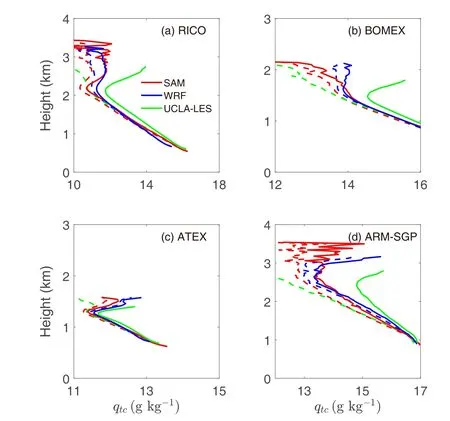
Besides convective core, two other types of plumes are provided, i.e., convective updraft, defined as plumes having liquid water and upward vertical velocity, and cloud,defined as grid points containing liquid water.Figures 10 and 11 show the mean profiles of vertical velocity and total water within convective updraft (solid lines) and cloud(dashed lines), respectively.The vertical velocity in the cloud plume either decreases or increases with height at a considerably smaller rate, which is less than half the vertical velocity in the updraft and convective core plumes.The decrease in total water with height in the cloud plume is slightly larger than that in updraft, which in turn is greater than in convective core.This is consistent with the larger entrainment rate within cloud and updraft plumes (Wang and Zhang, 2014).Comparison of Figs.10 and 11 shows that, for different types of plumes, the difference in simulated vertical velocity is greater than the difference in total water across the models.

These results suggest the need to distinguish between different types of plumes in the parameterization of shallow convection, since they have very different properties.For example, convective core may be more relevant to convectivescale transport, convective updraft may be more relevant to condensation, and the cloud plume is more relevant to radiation.These conditionally sampled variables thus shed light on the pathways toward further development of convection schemes by considering multiple plume types.

3.4.Model sensitivity to SGS turbulence scheme

To see to what extent the differences in model behavior are due to the choice of SGS turbulence scheme, we carry out sensitivity experiments by using the Smagorinsky-type turbulence scheme with the Smagorinsky coefficient set to 0.15 in SAM and WRF.Figures 12 and 13 show the mean profiles of the convective core fraction and the diagnosed entrainment rate for the four cases, with the Smagorinsky-type simulations in SAM and WRF superimposed.As can be seen,the change of SGS turbulence scheme does not yield significant differences in all cases except ATEX, where the Smagorinsky-type closure tends to produce less cloud compared to the 1.5-order TKE closure (Fig.12c).This is mainly due to the weaker mixing near the stratocumulus top.If we increase the Smagorinsky coefficient from 0.15 to 0.17, the differences between simulations using Smagorinskytype closure and 1.5-order TKE closure are almost indistinguishable (not shown).This suggests that the difference in SGS turbulence scheme is not directly responsible for the differences in model behaviors.It is more likely that other factors, such as technological details in the framework, advection, diffusion, damping, and, more importantly, their interactions, are responsible for the differences.This also highlights the need to use different LES models to reduce model dependencies.

Fig.8.Convective core ensemble averages of vertical velocitywc(dashed) and total water qt (solid) for the cases of (a) RICO, (b)BOMEX, (c) ATEX, and (d) ARM-SGP, simulated by SAM(red), WRF (blue), and UCLA-LES (green).The black lines indicate the MMM, and the gray shading denotes the width of twice the standard deviation of the results of all LES models.

Fig.10.Convective updraft (solid lines) and cloud (dashed lines)ensembleaveragesofverticalvelocitywc for the cases of(a)RICO,(b) BOMEX, (c)ATEX,and(d)ARM-SGP,simulated by SAM(red),WRF (blue), and UCLA-LES (green).

Fig.11.As in Fig.10 but for convective updraft (solid lines) and cloud(dashed lines) ensemble averages of total water qtc

Fig.12.Profiles of the convective core fraction for the cases of (a)RICO, (b) BOMEX, (c) ATEX, and (d) ARM-SGP, simulated by SAM(red), WRF (blue), and UCLA-LES (green).Solid lines stand for simulations with the 1.5-order TKE turbulence scheme, while dashed lines stand for simulations with the Smagorinsky-type turbulence scheme in SAM and WRF.

Fig.13.As in Fig.12 but for fractional entrainment rate.

4.Data records and usage notes

This dataset, simulated by the large eddy models SAM,WRF, and UCLA-LES, for four shallow convection cases,has been submitted to Zenodo and is available at https://doi.org/10.5281/zenodo.7895982.The dataset format is version 4 of the Network Common Data Form (NetCDF),which is easy to read and written by professional common software such as Climate Data Operators (CDO,https://code.mpimet.mpg.de/projects/cdo), NCAR Command Language (NCL, http://www.ncl.ucar.edu), NetCDF Operator (NCO, http://nco.sourceforge.net), and Python (https://www.python.org).

For each convection case, there are 19 2D variables (as is shown in Table 2), including winds, temperature, and specific humidity.Conditionally sampled variables, such as incloud temperature, total water, and vertical velocity, are also provided, which are indispensable for calculating entrainment rates.Besides convective core, two other types of plumes are provided, i.e., convective updraft, defined as plumes having liquid water and upward vertical velocity,and cloud, defined as grid points containing liquid water.The dataset presented in this study can be used for validation of the parameterization of shallow convection and may provide guidance for further development of convectionschemes by considering multiple plume types.

Table 2.List of the LES output variables.

5.Summary

This paper describes a dataset simulated by the three large eddy models SAM, WRF, and UCLA-LES, for four shallow convection cases (RICO, BOMEX, ATEX, and ARM-SGP), which vary in inversion strength.The general features of the model output are presented, and the data records and usage notes are provided.Results show that the different LES models show similar performance for each case, albeit with noticeable differences manifested in the horizontal winds.The MMM and the standard deviation of the results of all LES models are also given.If all models produce similar features, this means the standard deviation between the models is small, so their average can be taken as the“ground truth”.If the models show greater diversity in some features, then their mean plus/minus the standard deviation yields an acceptable range for that field.Sensitivity experiments show that the differences of the SGS turbulence scheme are not directly responsible for the differences in model behavior.Other factors, such as technological details in the model framework, are more likely to matter.

Compared to SAM and UCLA-LES, the WRF model appears to be more efficient in transporting moisture to upper levels, leading to a wetter free atmosphere and drier boundary layer.SAM tends to simulate a higher cloud top than WRF and UCLA-LES, due to the fact that SAM produces a larger variance of vertical velocity within the CBL, which helps clouds to penetrate progressively deeper.Conditionally sampled variables, such as in-cloud moisture and vertical velocity, are also analyzed, which are indispensable for calculating entrainment/detrainment rates.All models show that the entrainment rate decreases with height in all cases except ATEX, where a secondary peak appears near the cloud top.Given that the entraining/detraining process is central to the parameterization of cumulus convection (Sun,2009; Lu et al., 2011, 2012, 2013), the dataset presented in this study is potentially useful for validating and improving such parameterization schemes.

Acknowledgements.The authors thank the two anonymous reviewers for their constructive comments, which certainly helped to clarify and improve the original paper.This work was jointly supported by the National Key R&D Program of China (Grant No.2021YFC3000802) the National Natural Science Foundation of China (Grant No.42175165), and the National Key Scientific and Technological Infrastructure project “Earth System Numerical Simulation Facility” (EarthLab).

Open AccessThis article is licensed under a Creative Commons Attribution 4.0 International License, which permits use, sharing, adaptation, distribution and reproduction in any medium or format, as long as you give appropriate credit to the original author(s)and the source, provide a link to the Creative Commons licence,and indicate if changes were made.The images or other third party material in this article are included in the article’s Creative Commons licence, unless indicated otherwise in a credit line to the material.If material is not included in the article’s Creative Commons licence and your intended use is not permitted by statutory regulation or exceeds the permitted use, you will need to obtain permission directly from the copyright holder.To view a copy of this licence,visit http://creativecommons.org/licenses/by/4.0/.

Fig.S1.Regressed (a) March and (b) April surface air temperature anomalies (units: °C) against PC1 in the CESMLENS simulation.(c-d) Same as in (a-b) but for the regressed precipitation anomalies (units: mm d-1).Values significant at the 95% confidence level are dotted.

Fig.S2.Distribution of the prescribed SST anomalies in (left) February, (middle) March, and (right) April in CAM5_NASST.

Fig.S3.Same as in Fig.S2 but for the prescribed SST anomalies in CAM5_TIOSST.

Fig.S4.Distribution of the diabatic forcing (units: K d-1) in LBM_NEASC.The left panel shows the horizontal distribution of the diabatic forcing, and the right shows the vertical profile of the diabatic forcing at the center of the forcing area.

Fig.S5.The standardized PC1 (bar) and the hindcasted PC1 (red line) based on the leave-one-out cross-validation method during 1961-2020.The hindcasted PC1 is constructed by the February NASSTI, TIOSSTI, and NEASDI.