Regional rural transformation and its association with household income and poverty incidence in Indonesia in the last two decades

Tahlim SUDARYANTO, ERWIDODO, Saktyanu Kristyantoadi DERMOREDJO, Helena Juliani PURBA#, Rika Reviza RACHMAWATI, Aldho Riski IRAWAN

1 Research Center for Behavioral and Circular Economics, National Research and Innovation Agency (BRIN), Jakarta 12710,Indonesia

2 Research Center for Economics of Industry, Services and Trade, National Research and Innovation Agency (BRIN), Jakarta 12710, Indonesia

3 Indonesian Center for Agriculture Socio-Economic and Policy Studies, Bogor 16111, Indonesia

Abstract Increasing rural household income and reducing poverty rank among Indonesia’s top development priorities.Promoting rural transformation is one strategic policy framework to achieve these goals.In the last three decades, agricultural production has shifted from low-value food crops to high-value commodities, such as horticulture, estate crops, and livestock.Previous studies have analyzed rural transformation in Indonesia at the national level, but information on the magnitudes of impact across regions remains scarce.This study aims to analyze the changes in rural transformation at a regional level in the past two decades.The research utilizes secondary data from Statistics Indonesia (BPS), covering 34 provinces from 2000 to 2020, analyzed using descriptive and panel data regression analyses.The results show an increasing trend in the share of high-value agriculture (RT1) and rural non-farm employment (RT2).Both RT1 and RT2 are positively associated with the growth of rural household income and a lower poverty rate.However, the speed of structural transformation (ST), RT1, RT2, rural income growth, and poverty reduction vary across regions.This research implies that improving rural income and reducing poverty should be done by integrating policies, i.e., promoting highvalue agriculture and expanding rural non-farm employment.Particular attention should also be given to provinces with slow growth in ST, RT1, RT2, and rural household income.

Keywords: rural transformation, high-value agriculture, rural non-farm employment

1.Introduction

Indonesia has experienced rapid agricultural growth and rural transformation in the past three decades.Agricultural output value grew at an annual rate of 5.4%(Arifin 2013).While grain production has steadily grown since Indonesia reached rice self-sufficiency in 1984,the production of other commodities has grown much faster, particularly horticulture and estate crops (Hudoyoet al.2016).For example, egg production showed the highest growth of around 13% per year, followed by beef(10%), palm oil (9%), and orange (5.5%) (Sudaryantoet al.2021).In agriculture, the production of highvalue commodities, including livestock and fishery, has increased faster than food crops.Over the same period,rural laborers have been more engaged in non-farm employment (Sudaryantoet al.2021).

The national development plan in Indonesia has prioritized the improvement of rural household income and poverty reduction (BAPPENAS 2020).Given the dominant role of agriculture in the rural economy, increasing rural household income is often translated into increasing agricultural production (OECD 2020; Liet al.2020).Likewise, given the track record in achieving strategic development goals, research has focused much on the role of structural transformation (ST) (Kimet al.2018).However, the growth of ST in the past years has been slow,raising concerns in the formulation of the National Midterm Development Plan (RPJMN) 2020-2024 (BAPPENAS 2020).In fact, in relation to ST, rural transformation (RT)has attracted much interest from researchers in Asia(Berdegueet al.2014; IFAD 2016; Huang and Shi 2021).

In the context of Indonesia, Sudaryantoet al.(2021)analyzed the indicators and impact of RT at the national level.Using a similar concept, Erwidodoet al.(2021)reported the indicators and drivers of RT at the provincial level in East Java.Meanwhile, Susilowatiet al.(2021)reported the result of a case study using farm survey data in West Java.Past research has shown that indicators,drivers, and impacts of RT vary across regions (Huang and Shi 2021).Therefore, further examination is needed.Evidence of the RT impact is important for Indonesia as the characteristics across provinces and regions are diverse in terms of not only natural resources but also economic development and socio-culture.Therefore, a sound economic development framework should consider the concept of regionalization.

One concept of regionalization of Indonesia classifies the country into four regions, each with its own growth center (Nurhadi 2012): (i) Region A centered in Medan,North Sumatera; (ii) Region B centered in Jakarta;(iii) Region C centered in Surabaya, East Java; and(iv) Region D centered in Makasar, South Sulawesi.Economic development in the growth center is expected to encourage development in other provinces in the same region.This concept is based on the location theory’s framework and the growth pole.However, it should be noted that each region’s economic development priority may differ.

Understanding the dynamics of RT in each region is essential to formulate a sound and contextual policy framework.Therefore, this paper aims to identify RT’s indicators and their associations with rural household income and poverty incidence at the regional level, using data from all provinces of Indonesia.We construct a typology of the corresponding regions according to the relation between ST, RT, and rural household income and poverty incidence.

The remainder of the paper is organized as follows.Section 2 presents the methodology, i.e., data sources,measurement, and analytical approaches.Section 3 presents the results and discussions.Section 4 concludes the study and provides the policy implications.

2.Data and methods

2.1.Data

This study uses Statistics Indonesia (BPS) databases and publications from 2000 to 2020, which include the general statistics, the state of the labor force in Indonesia,the calculation and analysis of Indonesian macro poverty,and income statistics.Another dataset used in this study is the time-series data of the gross domestic product(GDP) from 2000 to 2020 from each province and sector,including the GDP of agriculture (nominal).Table 1 presents more detailed definitions of the variables.

Table 1 Definition and measurement of variables

The employment data were collected from the Indonesian Workforce’s publications issued twice a year in February and August.This study uses employment data collected in August from 2000 to 2020 to reflect the mid-year employment data.The poverty data were collected from BPS (https://www.bps.go.id/subject/23/kemiskinan-dan-ketimpangan).The concept to determine poverty is the ability to meet basic needs as stipulated in the Handbook on Poverty and Inequality published by the World Bank.BPS publishes the poverty data twice a year, in March and September.Consistent with the employment data, this study uses the September poverty data to reflect the mid-year poverty.Finally, the regional classification is based on the concept of growth center with the A, B, C, and D notations explained in Table 2.

2.2.Methods

This paper utilizes both quantitative and qualitative analyses.The former includes calculating the descriptive statistics and running an econometric analysis.The results of descriptive statistics are presented in graphs or tables.Several indicators included in this study are shares, trends, and average growth, including the nonfarm GDP, rural non-farm employment, rural household income, and the share of high-value commodities.These variables are compared across regions based on the mean difference test.The provinces’ economic growth rates are classified into fast and slow based on the median value.

The median is a statistical measure representing the middle value in a dataset when the data are arranged in ascending order.Unlike the mean, the median measures the central tendency resistant to outliers.This means the median is a better measure of a dataset's ‘typical’ value when a few extremely large or small values could skew the average.First, the data are arranged in numerical order.Then, the middle value is identified to determine the median.The median is the middle value if the dataset has an odd number of values.In the case of an evennumber, the median is calculated by taking the average of the two middle values.Therefore, for the analysis of this study, the formula becomes:

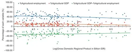
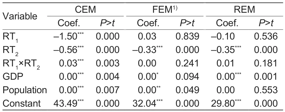
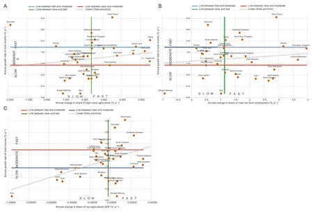
Slow

Meanwhile, the rural household income and poverty rate are classified into fast, moderate, and slow.A standard deviation is used to determine the limits of these three categories and the data diversity.Since half of the standard deviation determines the slow and fast limits, the formula to determine the limit is:

Slow<(Median-0.5×Standard deviation)

(Median-0.5×Standard deviation)≤Moderate≥(Median+0.5×Standard deviation)

Fast>(Median+0.5×Standard deviation)

A panel data regression analysis is used to analyze the association between the share of high-value agriculture(RT1) and the share of rural non-farm employment (RT2)and the rural household income and poverty incidence.In general, the formula for the panel data regression model is:

whereidenotes the number ofkcross-section units,tdenotes the time, andprepresents the explanatory variables.

It is realized that there is an issue of endogeneity related to some variables, particularly RT1and RT2.Therefore, the estimated parameter of the above regression is interpreted as an association rather than causality.When estimating the panel data regression,the parameter estimation method highly depends on the assumptions about the intercept, slope, coefficient,and error.The three-parameter estimation models from the data panel are common effect model (CEM), fixed effect model (FEM), and random effect model (REM).The suitable model is selected by performing a series of statistical tests, namely Chow, Hausman, and Lagrange multiplier (LM).The Chow Test compares the best or the most appropriate model between CEM and FEM; the Hausman Test compares FEM and REM; and the LM Test compares CEM and REM.If one model is selected consecutively in two different tests, then the model is considered the most suitable.

(1) Chow test:

H0:μ1=μ2=μN-1(There is no difference in individual effects, or the common effect model is better than the fixed effect model; whereμis individual effects).

H0:minimumμi≠0 (There are differences in individual effects, or the fixed effect model is better than the common effect model).

RejectH0ifP-Value (P-test)<0.05.

(2) Hausman test:

H0:Cov(μit,Xit)=0 (There is no correlation between individual error and explanatory variables, or the random effect model is better than the fixed effect model; whereμis individual error;Xdenotes explanatory variables).

H1:Cov(μit,Xit)≠0 (There is a correlation between individual errors and independent variables, or the fixed effect model is better than the random effect model).

RejectH0ifP-Value (P-test)<0.05.

(3) LM test:

H0:σμ2=0 (There is no relationship between composite errors, or the common effects model is better than the random effect model; whereσ iscomposite errore).

H1:σμ2≠0 (There is a relationship between composite errors, or the random effect model is better than the common effect model).

RejectH0ifP-Value (P-test)<0.05.

3.Results and discussion

3.1.Indicators of rural transformation at the national and regional levels

Understanding the nature and dynamics of agricultural GDP and employment at the macro level is needed to realize a structural transformation (ST) from an agriculture-dominated to a non-agriculture-dominated economy (Jayneet al.2019).This common path has been observed in many countries and indicates economic progress.However, Fig.1 shows significant gaps between agricultural GDP and labor shares in several provinces.The disparity is primarily due to an increase in agricultural output but with a lower relative worth.In addition, activities in the non-farm sectors increase along with a higher demand for processed products with fewer agricultural products.This indicates that agriculture’s contribution continues to decline.Although the agriculture sector accounts for a significant portion, it is becoming less significant in the country’s economy (Arendonk 2015).

Fig.1 Convergence of agricultural GDP shares and employment in 2000-2020 at the provincial level.

Fig.1 indicates that several provinces have a significant gap between the share of agricultural GDP and rural agricultural employment.This is due to the role of the agriculture sector as the main source of employment for the rural community.From 2000 to 2020, there was a convergence in the decreased agricultural GDP and employment shares, which shows that the non-agricultural sector grew more rapidly.The smaller (converged) gap shows that agricultural labor’s productivity is close to nonagricultural labor.Therefore, a policy aiming to increase farmers’ income should improve, among others: (a) the opportunity for labor to work in the non-agricultural sector,(b) the opportunity to increase farmers’ income through labor productivity, and (c) the opportunity to increase labor wages in rural areas.

At the national level, RT1increased significantly between 1990-1999 and 2000-2009, from 40.6 to 49.2%(Sudaryantoet al.2021).This shows that in the 1990s and 2020s, the composition of agricultural production moved from staple food and low-value products to highvalue and more commercial commodities (horticulture,estate crops, and livestock).This transformation indicates changes in farmers’ orientation from subsistence to market-driven.Meanwhile, the nearly stagnant trends of commercial products in the 2010s reflect the government’s priorities on food crop production.

The findings by Sudaryantoet al.(2021) show that from 1990 to 1999, agriculture was still a primary source of employment.However, between 2000 and 2009, the trend was reversed when the non-farm sector accounted for 58.1% of total employment and rose steadily to 66.1%in 2010-2019.In addition, the rapid urbanization and development of the non-farm sectors, particularly the service sector, opened new employment opportunities.At the regional (provincial) level, the changes illustrate the occurrence of RT.The dynamic changes in RT1and RT2at the regional level are discussed in more detail as follows.

Based on the regional GDP data, nationally and regionally, the share of high-value output (RT1) in the total agricultural production in 2000-2020 was greater than the share of food crop production as a staple food (Fig.2).The share of high-value commodities continued to increase throughout the year, and the share of food crop decreased.This figure indicates that ST occurs at the national and regional levels.As shown in Fig.3, the high-value share in Region A is the largest among the other three regions.Likewise, the share of high-value output is higher than food crops, almost three times in Region A.As shown in Appendix A, the statistical test confirms that RT1in Region A is larger than Region B (with aP-value of 0.0846) and Region D (with aP-value of 0.0075).Region A, with the growth center in Medan, shows a higher level of RT1,which could be attributed to the dominance of estate crops and government support for the palm oil industry.In fact,Region A is the main contributor to establishing Indonesia as the world’s largest producer and exporter of palm oil.Meanwhile, RT1in Region B is not significantly different from Regions C and D, but RT1in Region C is significantly larger than Region D.The dominant commodities in Region D, located in the eastern part of Indonesia, are livestock, estate crops, and food crops.

Fig.2 Share of high-value commodities and food crop production across regions (%) in 2000-2020.

Fig.3 Share of rural farm (F) and non-farm (NF) employment in 2000-2020.

The agriculture ST generally implies a gradual increase in farm sizes and a reallocation of the agricultural workforce to other sectors (Huang 2018).ST is also often driven by agricultural innovations and new job opportunities in manufacturing and services (Chrisendoet al.2021).

Fig.3 shows the share of rural non-farm employment(RT2) as the second indicator of RT in the four main development areas.Overall, the trend increased in 2000-2020.Regions A, B, and C indicated a similar level of RT2, around 68.6-70.2% in 2020, with insignificant statistical differences.However, in the less developed Region D, the level of RT2was significantly lower than in Region A (P-value 0.0002), Region B (P-value 0.0026),and Region C (P-value 0.0001).Economic development in Eastern Indonesia (including Region D) is lagging compared to other regions.According to the Ministry of Villages, Development of Disadvantaged Regions, and Transmigration, 84% of 122 disadvantaged regions are in Eastern Indonesia.The lack of infrastructure is a major development constraint in this region.For instance, 3% of the villages in the region do not have access to electricity.

Fig.4 compares rural household income across regions in 2000-2020.Household income showed an increasing trend in all regions.Surprisingly, Region D, which is in an earlier stage of economic development, showed a higher household income per capita than the other three regions (statistically significant with aP-value of 0.000).However, the per capita household income in Region A does not significantly differ from that in Regions B and C.The highest income in Region D is due to the abundant natural resources (land and mineral resources) but a lower population density.Infrastructure improvement supporting rural transformation is also associated with improving household income.Households with improved access to rural infrastructure have more opportunities to diversify their incomes (Reardon 2015; Teame and Woldu 2016 ).Internet access and other infrastructures are essential.Rural households can utilize these infrastructures for e-commerce activities and earn more income.The investments in Internet infrastructure and human resources for e-commerce development in rural areas increase the ‘digital dividend’,hence the rural income.Therefore, policymaking on rural e-commerce should prioritize the empowerment of impoverished communities (Penget al.2021).

Fig.4 Comparison of rural household incomes across regions in 2000-2020.

Fig.5 shows that the poverty rate declined in all regions in the period of 2000-2020.Region D exhibits a higher poverty rate than the other three regions(statistically significant with aP-value of 0.0000).Regions A and B do not significantly differ.Region B shows a higher poverty rate than Region C (statistically significant with aP-value of 0.0000).

Fig.5 Poverty rate across regions (%) in 2000-2020.

The above-mentioned observation is contradictory to the evidence in Fig.5, which shows that Region D earned the highest household income.A plausible explanation for this fact is the wider income inequality in this region,as shown by Erwidodoet al.2021.Region D, located in the eastern region of Indonesia, is included in the group from disadvantaged areas (Sholeh 2014).Inequal development among regions means low accessibility of economic and social facilities and infrastructure services,which inhibits regional economic growth (Reardon 2015;Erwidodoet al.2021).Inequality also creates pockets of poverty in remote, isolated, critical, and resource-poor regions, which creates gaps between regions (Ginting 2015).Furthermore, Region D mostly grows food crops(rice, maize, and soybean) as a source of livelihood,whereas Region A mostly grows estate crops (highvalue commodities).Region C grows food crops, but the mechanization of agriculture and the implementation of food estates in several locations in Kalimantan seems to have contributed to poverty reduction in the region (Soleh 2014; Jayneet al.2011).

Agricultural growth remains a practical approach to poverty alleviation, particularly in rural regions.Evidence suggests that agricultural growth increases income for 40% of the poorest people (Fan and Cho 2021).Independent farming is the most important source of income for rural households, followed by activities outside the agriculture sector.Self-employed and salaried work of non-farm origin account for a third of farmers’ income, but these activities do not involve all households.From the income sources, less poor households derive 40% of their income from non-farm activities.In contrast, they account for only 10% of the income of the poorest households(Schwarze and Zeller 2005).

3.2.Association between RT and rural household income

This section presents the result of an econometric analysis that investigates the association between RT and rural household income.The model also includes other explanatory variables, such as GDP and population.The study also performs Chow and Hausman tests to assess the robustness of the results.Three analyses, i.e., CEM,FEM, and REM, examined the relationship between rural household income and various independent variables.The dependent variable in all three analyses is rural household income, while the independent variables are RT1, RT2, the interaction between RT1and RT2(RT1×RT2),GDP, population, and a constant term.The results of CEM analysis indicate that RT2has a statistically significant positive association with rural household income (Coef.5 801.8,P>tis 0.034), as well as (RT1×RT2)(Coef.561.4,P>tis 0.041).On the other hand, RT1,GDP, and population do not show a statistically significant association with rural household income (Table 3).

Table 3 Results of common effect model (CEM), fixed effect model (FEM), and random effect model (REM) panel data regression of rural transformation (RT) on rural household income

The results of the FEM analysis reveal that RT2has a statistically significant positive association with rural household income (Coef.28 496.6,P>tis 0.000).Similarly,RT1, (RT1×RT2), and population also demonstrate a statistically significant association with rural household income.However, GDP does not significantly affect rural household income.Meanwhile, the REM analysis shows similar results to the CEM analysis, which indicate that RT2has a statistically significant, positive association with rural household income (Coef.5 801.8,P>tis 0.032), along with(RT1×RT2) (Coef.561.4,P>tis 0.039).Similarly, RT1, GDP,and population also show statistically significant, positive associations with rural household income.

The most suitable parameter estimation model of the association between RT1, RT2, GDP, and population with rural household income concludes that FEM is the most appropriate.The results in Table 3 show that RT2, GDP,and population are significantly and positively associated with household income in rural areas.This is most likely due to the availability of non-agricultural employment,which includes labor-intensive work with higher wages than in the agricultural sector.In this case, creating nonagricultural job opportunities would be a better alternative to increase the income and welfare of farmers and rural households.Similar to RT2, the regression results of the association between RT1and rural household income indicate a positive association, albeit insignificant.This suggests the higher potential of high-value commodities production in that region to contribute to rural households’income than low-value commodities.

The coefficient of GDP is 0.2, and it is marginally significant at the 0.05 level.As reflected by GDP,economic growth may provide employment opportunities,investment, and market expansion, leading to higher income for rural households.The positive association between GDP and rural household income indicates the importance of macroeconomic policies and strategies that foster sustainable economic growth for rural development.

Lastly, the coefficient of the population is 57.8, which is statistically significant at the 0.05 level.This finding aligns with the literature emphasizing the positive relationship between population growth and rural income.A larger population means a larger consumer base and demand for goods and services, stimulating economic activities and boosting income in rural areas.In addition,population growth may also lead to increased labor supply, which contributes to agricultural and non-farm sectors’ productivity, boosting rural household income even further.This finding suggests the importance of population dynamics and demographic trends in formulating rural development policies.

3.3.Association between RT and poverty incidence

Panel data regression analysis was also conducted to analyze the association between RT1and RT2and the poverty rate in rural areas.Hypothesis testing to select the most appropriate parameter estimation model shows that FEM is the chosen model, as shown in Table 4.The table shows that RT2is significantly and negatively associated with poverty rates in rural areas.The higher the RT2, the smaller the level of poverty in rural areas.A one percent increase in RT2will likely be associated with a reduction of the poverty level in rural areas by 0.33 percentage points.This result is understandable because expanding rural nonfarm employment will increase rural household incomes above the poverty line.This is in line with the research conducted by Li and Zhang (2013), which suggests that off-farm employment plays a crucial role in reducing poverty in rural China.The study indicates that higher engagement in non-agricultural jobs lowers the probability of experiencing poverty and increases the probability of escaping poverty.The regression results show a statistically non-significant association between RT1and the poverty rate in rural areas.

Table 4 Results of common effect model (CEM), fixed effect model (FEM), and random effect model (REM) panel data regression of rural transformation (RT) on poverty incidence in rural areas

The coefficient of GDP is limited to zero, indicating that a one million Indonesian Rupiah (IDR) increase in GDP is not associated with any change in poverty incidence.Similarly, the coefficient of the population is also limited to zero, suggesting that a 1 000-person increase in population does not lead to any change in poverty incidence.These results imply that changes in GDP and population are not directly associated with the poverty rates in Indonesia.

3.4.Typology of RT by region

Fig.6-A shows a positive association between RT1and rural household income, especially if RT1reaches more than 50%, but varies across regions.This trend occurs in most provinces in Indonesia.Region D is lagging compared to the other three regions.Increases in rural income may vary significantly across regions depending on other factors, such as local economy, natural resources, infrastructure, and market access (Sjafrizal 2012).For example, rural areas with strong agricultural industries may experience faster income growth.In addition, rural areas with access to transportation networks, telecommunications, and other modern amenities may also have an advantage in attracting businesses and facilitating economic activities, leading to higher household incomes (Reardon 2015).

Fig.6 Relationship between RT1, RT2, non-agricultural GDP, and rural income across regions, 2000-2020.Poly.(A)=Polynomial estimation of region A; Poly.(B)=Polynomial estimation of region B; Poly.(C)=Polynomial estimation of region C; Poly.(D)=Polynomial estimation of region D.

RT2is also positively associated with higher incomes in rural areas.However, the distribution is relatively spread out, as shown in Fig.6-B.This observation implies that the priority of development should not only focus on producing high-value commodities but also promoting rural non-farm employment.Fig.6-B also shows that rural income increases when the RT2is around 30%.There are many ways to promote rural non-farm employment,such as developing small businesses, expanding existing companies, or establishing new industries.Other strategies include investing in infrastructure, education,and training programs to help rural residents acquire the skills and knowledge they need to participate in the workforce.

The increase in RT2is also consistent with the increase in the non-agricultural GDP, which leads to the increase in rural income, as shown in Fig.6-C.The three variables,i.e., RT1, RT2, and the share of non-agricultural GDP,show a positive relationship with household income in rural areas.This analysis also shows that the higher the three variables, the higher the rural income.However, the picture above indicates that the three variables are not synchronized in some provinces.

Fig.7 show the positive relationship between the speed of RT, structural change, and rural income growth.Provinces experiencing faster RT1typically experience a faster increase in rural income, above a 0.4% annual growth rate (Fig.7-A).This observation is prevalent in provinces on Java Island.The same trend occurs when the industrial centers in the Java regions only have a marginal influence on the growth of non-farm labor.Nevertheless, this condition raises incomes in rural areas.In contrast, in some provinces, rural income growth tends to decrease along with the rapid acceleration in RT2,such as in West Nusa Tenggara, West Sulawesi, North Kalimantan, East Kalimantan, West Papua, and East Nusa Tenggara.This evidence means that the rapid acceleration of RT2decreases rural income growth.

Fig.7 The annual growth rate of rural income and annual change in RT1, RT2, and non-agricultural GDP, 2000-2020.

Faster structural change is also positively correlated with regional rural incomes (Ryandiansyah and Azis 2018), especially when the GDP growth is above 3% per year.The acceleration of incomes in rural areas in the Java provinces is sufficient to accelerate the economy to less than 2% per year.At the same time, most provinces are located to the right of the median, which means that increasing rural incomes demands more than 2 percent of annual non-agricultural GDP growth.

Based on Fig.7, a typology analysis was conducted focusing on the speed of ST, RT, and the growth rate of rural income.The rural and structural transformation data divide all provinces into two groups (ST and RT,fast and slow).Meanwhile, rural income growth is divided into three groups (rapid, average, and slow)(Birthal and Pandey 2020).The structural transformation used the median annual percentage change in all provinces from 2000 to 2020 as a dividing point to identify which provinces are categorized into fast and slow groups.The sample provinces were grouped into fast and slow RT provinces based on RT1and RT2by the same method.The medians of RT1and RT2are 2.41 and 1.14%, respectively.According to the annual average rural income growth, the three categories in rural transformation are: fast, moderate, and slow.Eight provinces are in the fast category, with a more than 8.02%growth rate.Meanwhile, 14 provinces are in the moderate category with a growth rate of 7.23 and 8.02%, and ten other provinces are in the slow category with a less than 7.23% growth rate.The results of the typology analysis on RT1and RT2are presented in Appendices B and C.

There are interesting observations about the speed of RT1, RT2, ST, and the growth of rural incomes.First,there is no province with a fast increase in rural income without slow ST and RT1(the bottom left corner is empty in Appendix B).Second, almost all of the fast ST and RT1(fast and slow) categories are filled by 16 provinces,meaning that the 17 provinces need to increase the nonagriculture GDP.Third, some provinces have fast RT1but show rapid rural income growth despite a slow GDP growth(1 province).Fourth, all provinces fall under almost all ST,RT2, and rural income categories except Slow ST, Slow RT2, and Slow rural income.Fifth, the provinces in Java,Bali, DI Yogyakarta, South Kalimantan, and Riau Islands need to increase the speed of rural income growth to slow the speeds of ST and RT2.Finally, in the provinces of Banten, West Java, Central Java, and East Java, the rural income growth is relatively moderate with ST and RT2.

The relationship between the share of nonagriculture GDP,RT1, RT2, and poverty rate across provinces is presented in Fig.8.Regardless of variation across regions, the poverty rate tends to decline with the increase in RT1.A similar pattern is observed in the relationship between the share of RT2and the change in the poverty rate.

Fig.8 The annual change of poverty rate and annual change of RT1, RT2 and non-agricultural GDP, 2000-2020.

Based on the speed of the changes in ST, RT1, and the poverty rate, East Java and North Maluku provinces are categorized as fast speed, whereas North Sumatra and North Kalimantan are classified as low speed (Appendix D).On the other hand, based on the speed of changes on ST, RT2, and the poverty rate, Central Sulawesi, South Sulawesi, West Sulawesi, and North Maluku are categorized as fast speed.In contrast, the Bali and North Kalimantan provinces belong to the low-speed group (Appendix E).

3.5.The driver of RT (IPIs)

Huang (2018) summarized that the three major drivers of RT are institutions, policies, and investment (IPIs).The following section briefly describes the significant IPIs of RT in Indonesia at the national level and highlights them in some regions.

InstitutionsStrengthening farmers’ groups and partnerships between smallholders and large companies are among the significant institutions contributing to RT.This scheme is recorded as a successful case in the estate crops and poultry sectors and contributes to the commercialization of the sectors.Another institutional arrangement is the promotion of farmers’ groups and the federation of farmers’ groups, which was started during the early stage of the green revolution and has contributed to the achievement of rice self-sufficiency and agricultural diversification toward high-value commodities.

There is no institutional arrangement in the land market, which leads to land market transaction expansion.However, the government has allocated some state lands to smallholder farmers, particularly in the estate crop sector.This policy has increased farm size and expanded the production capacity of related agricultural commodities, including high-value crops.

PoliciesSignificant policies dedicated to agriculture are derived from the Food Law Number 18/2012 mandated to achieve food self-reliance and food sovereignty.Furthermore, the Strategic Plan of the Ministry of Agriculture for 2020-2024 underlines that food security continues to be a strategic agricultural development goal(Huang and Rozelle 2018).In practice, this policy goal is translated into self-sufficiency in staple and strategic commodities such as rice, maize, soybean, sugar, beef,chili, and onion.

Primary policy instruments at the farm level to achieve this goal are (a) government purchase prices (Harga PembelianPemerintah, HPP) for rice and sugar; (b)fertilizer subsidies, seed subsidies, and credit (interest rate subsidies and credit guarantees); (c) grants of machinery to farmers group; and (d) extension services.Furthermore, general support for agriculture includes irrigation infrastructure, research and development (R&D),marketing, and promotion (OECD 2020).Agricultural R&D in the Ministry of Agriculture is supported by 1 537 scientists in the diverse field of expertise, and national research centers spread over all provinces in the country.According to Liet al.(2021), important factors to consider are the declining contribution of agricultural input growth to output growth, the significance of fertilizer and machinery inputs, the fluctuation of total factor productivity (TFP)growth influenced by agricultural policies, the necessity for government assistance, the type of agricultural output growth driven by technology innovation, and the regional characteristics of TFP growth.

Trade policy measures include tariffs, non-tariff barriers(quantitative limits, import licensing, SPS requirements),and variable export taxes (for CPO and cocoa beans).These policies significantly increased the Producer Support Estimate (PSE) from 7% in 2000-2002 to 24%in 2019-2021 (OECD 2022).In addition, significant policies in the non-farm sectors are (a) the development of small-scale agroindustry in the rural areas and (b) the promotion of small and medium enterprises (SMEs) in both agriculture and non-farm sectors.

InvestmentInvestment, i.e., incremental capital, is also a supply factor in economic development, and its effectiveness largely depends on another supply factor,namely labor.An expansion of capital through investment may increase output only if additional laborers are available, and an industry upgrade may contribute to growth only if human resources for the current labor force are enhanced.Consequently, supply-side factors have a more significant impact on long-term growth.Sustained long-term growth is primarily a continuous argument for production capacity or an outward shift of the production frontier.Demand-side factors may indirectly stimulate the out-shifting of the production frontier, as they may stimulate technological progress and capital investment(Diaoet al.2010).However, stimulating the outward shift of the production frontier is distinct from bringing actual production up to the frontier, and other supply-side factors may have more direct and practical effects on expanding production capacity and, thus, on sustained long-term growth (Zhonget al.2013).

In the early green revolution, the accelerated growth of agricultural production, particularly rice, was driven by the introduction of high-yielding varieties (IR5 and IR8) and investment in irrigation.The construction of dams, reservoirs, and irrigation canals in the early stage was funded by the World Bank and continued by the government funds in the subsequent periods.During 1980-1989 total irrigated area increased by 1.45%, and 1.53% during 1990-1999.However, during subsequent periods, the growth of irrigated areas decreased by 0.83%in 2000-2009 and -2.2% during 2010-2020.

Comparison across regions indicated that the share of irrigated areas in regions A, B, and C is relatively higher (23.8% in 2000 to 27.4% in 2022) than in region D (19.6% in 2000 and 18.0% in 2022).Better irrigation infrastructures in regions A, B, and C explain the relatively higher share of high-value commodities production in these regions.Another notable government investment was in the construction of road infrastructures.During 1993-1997 road construction in the rural regions was regulated by the Presidential Decree on Isolated Rural Regions, which mandated building rural infrastructure,including rural roads.Massive road infrastructure development has also been significant during 2014-present.This development has contributed to the transformation toward more market-oriented economic activities, including the production of high-value commodities and rural non-farm sectors at both on-farm and off-farm segments of the value chains (Reardon 2015;Bouet al.2018).Policymakers need to adopt a food system approach that considers trade-offs and aligns with other key objectives, such as food safety and ecological sustainability (Vos and Cattaneo 2021).

The rural transformation was also driven by investment in human resources, including complex (physical) and soft infrastructures.For example, in the past, physical infrastructures for the school building of elementary schools were based on a Presidential Decree related to elementary school development.On the other hand,soft infrastructures include developing a general and vocational education system.The intensity of human resource investment also varied across regions.For instance, in 2020, the number of elementary school buildings was the highest in Region C, at around 2 712 units, whereas, in Region D, the corresponding number was only 1 606 units.Comparable figures were also true for the Senior High School buildings, showing the highest number in Region C of 668 units, whereas, in Region D,the corresponding number was only 329 units.

4.Conclusion and implications

The declining share of agriculture GDP and share of agriculture employment tends to converge during 2000-2020, meaning that labor productivity in the agriculture and non-agriculture sectors are almost equal.This process is consistent with the evidence of rural transformation as indicated by the increasing trend of high-value agriculture production (RT1) and the share of rural non-farm employment (RT2).Furthermore, both RT1and RT2indicate a positive association with the growth of rural household income and the reduction of rural poverty incidence.

Based on the relationship between the share of agriculture GDP, the share of high-value agriculture, rural income, and the poverty rate, each province of Indonesia shows a different typology, which indicates different speeds of ST, RT1, RT2, rural income, and poverty reduction.The provinces of South Sulawesi and West Papua show fast speed in terms of ST, RT1, and rural income.On the contrary, the provinces of Aceh, North Sumatra, Riau, and West Kalimantan show slow speed in ST, RT1, and rural income.Furthermore, the provinces of South Sulawesi, Maluku, and West Papua indicate fast speed on ST, RT2, and rural income.In contrast, the provinces of West Sumatra and Riau show slow speed on ST, RT2, and rural income growth.

Based on the speed of the changes on ST, RT1, and the poverty rate, East Java and North Maluku provinces are categorized as fast speed.In contrast, North Sumatra and North Kalimantan are classified as low speed.On the other hand, based on the speed of changes in ST, RT2, and the poverty rate, the four provinces of Central Sulawesi,South Sulawesi, West Sulawesi, and North Maluku are categorized as fast speed, whereas the provinces of Bali and North Kalimantan are categorized as low speed.

The different typologies of ST, RT, rural income growth,and poverty rates across regions are associated with the different drivers, including institutions, policies, and investments (IPIs).Promoting institutions to strengthen farmers’ groups and partnerships contributes to significant agricultural growth, including high-value commodities.However, to some extent, a biased government incentive policy toward developing food crop sectors may have slowed the growth of high-value commodities.On the investment side, the varied intensity of infrastructure investment across regions partially explains the different typologies of ST, RT, rural income, and poverty rates in the corresponding regions.

The results of this research imply that accelerating rural household income and reducing poverty incidence should be done through an integrated policy, i.e.,promoting high-value agriculture and expanding rural nonfarm employment.Furthermore, regional development policy should emphasize the provinces in the slow-speed category regarding the growth in ST, RT1, RT2, rural income, and the reduction of poverty incidence.

Acknowledgements

The authors thank the Australian Center for International Agricultural Research for financial support (ADP-2017-024).Appreciation is also extended to project leaders and colleagues Prof.Chunlai Chen, Prof.Christopher Findlay,Prof.Jikun Huang, Dr.Dong Wang, and anonymous reviewers for their constructive comments.

Declaration of competing interest

The authors declare that they have no conflict of interest.

Appendicesassociated with this paper are available on https://doi.org/10.1016/j.jia.2023.11.029