Asset selection based on high frequency Sharpe ratio and robust correlation coefficient*

ZHANG Shanhua, ZHANG Sanguo

(School of Mathematical Sciences, University of Chinese Academy of Sciences, Beijing 100049, China)(Received 14 January 2022; Revised 14 April 2022)

Abstract High frequency Sharpe ratio, a measure of return and risk, is commonly used in current portfolio construction method since it can avoid covariance matrix in high dimensional analysis. The newly proposed D-SEV measures the correlation between stock’s return and high frequency Sharpe ratio index to further construct portfolio. However, there are some problems with the measure used in D-SEV, such as its lack of robustness and slow computational speed. In this paper, we propose to use a new correlation coefficient proposed by Sourav Chatterjee instead. The new correlation coefficient guarantee robustness, specifically it can reduce the impact of abnormal data on correlation, such as significant events that have a large impact on the asset prices. It is also extremely fast in its calculations. Extensive simulation demonstrate that new correlation coefficient outperforms D-SEV and other traditional methods in several different models. Actual Shanghai Securities Exchange (SSE) and Shenzhen Securities Exchange (SZSE) stock market data for 2019 and 2020 also show that the assets selected by new correlation coefficient earns 8% more excess annualized return than D-SEV, while it also owns a higher Sharpe ratio.

Keywords portfolio; high frequency Sharpe ratio; robust correlation coefficient

The portfolio is a classical problem of finance, which was fist addressed and solved by Markowitz[1]using mean-variance paradigm. This method is still used today as a standard method. The basis of the mean-variance model is to estimate the mean and covariance of the returns of underlying assets. Once the estimators are inaccurate, the results of the model will be very imprecise. Kan and Zhou[2]showed that the estimators of mean-variance paradigm have some shortcomings in the situation of large-scale mean-variance models. Michaud[3]proved that the error of expected returns by this model is over estimated. To solve these problems, extensive literature focus on improving the accuracy of estimator. For instance, the shrinkage estimation method is proposed by James and Stein[4]. Sharpe[5]and Chan et al.[6]impose a factor structure for the covariance among assets to reduce the number of free parameters of the covariance matrix. Other methods involve reduction of the dimension. Ao et al.[7]took advantage of LASSO to achieve dimension reduction. Chen and Yuan[8]provided a framework of portfolio selection under subspace and adopted factor model to achieve the global Sharpe Ratio. Although the aforementioned methods improved the original method from different aspects, there are still two problems to be solved. First, these methods employ long historical data, it is not compatible with the current rapidly changing market. The second problem is caused by the dramatic increase in the number of modern assets, the amount of assets facing by modern investors is much larger than traditional market. The essence of this problem is feature screening, it is first proposed by Fan and Lyu[9], they investigated the data for which the number of featurespis much more than the number of samplesnand propose a screening method called sure independence screening (SIS) to quickly reduce the ultrahigh dimension to suitable dimension . Following Fan and Lyu[9], the screening methods have been explored in two directions, Fan and Song[10]studied the specific model, Zhu et al.[11]and Liu et al.[12]did the research of model-free. However, the SIS methods have a premise: independent and identically distributed samples, which is invalid in the financial filed. To tackle these problems, Wang et al.[13]proposed an asset selection method based on high frequency Sharpe ratio and D-SEV, which do not need the assumption of identically distributed samples. They used D-SEV to calculate the correlation between stocks and high frequency Sharpe ratio, the variables here can be seen as a time series. Their method is reasonable because the D-SEV tells the proportion of the variance explained by the selected assets. Yet, it also has two disadvantages, the lack of robustness and the high computation cost. To deal with these issues, we propose to introduce the robust correlation coefficient instead of D-SEV to evaluate the correlation between assets and high frequency Sharpe ratio index. Simulations and empirical analysis show that our method outperforms D-SEV and other traditional method in several different situations.

1 High frequency Sharpe ratio index

1.1 Sharpe ratio

Sharpe ratio, proposed by Sharpe[5], is a well-accepted measure of assets in financial field, defined as

(1)

whereRfis the annualized risk-free interest rate and is commonly set as benchmark,σpis the standard deviation of annualized return of portfolio, andE(Rp) is expected annualized rate of return of portfolio.

The Sharpe ratio is a measure of excess return earned over the risk-free rate return for every unit of risk taken. High risk return is the ultimate goal for portfolio construction. It can be seen that high Sharpe ratio leads to high excess return earned for a given amount of risk.

1.2 High frequency Sharpe ratio

With the development of high frequency data, high frequency stock volatility can be calculated as a proxy for the standard deviation. Integrated volatility can be defined as

(2)

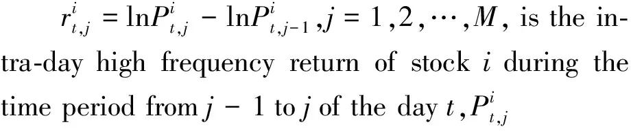
Consider stocki=1,2,…,p, for the dayt=1,2,…,T, high frequency Sharpe ratio of this stock is defined by the daily data of the stock prices and market index yield:

(3)

HereRi,tis the yield of the stockiduring dayt,Rm,tis the market index yield during daytas the benchmark, here we choose market index yield instead of risk-free rate return. Because our portfolio contains stocks only, our benchmark can only contain stocks as well, RVi,tis the integrated volatility as described above.

1.3 Choose assets to construct a return time series of an index

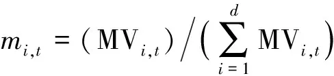
Similar as original Sharpe ratio, stocks with higher high frequency Sharpe ratio can also be considered as an indication of better performance. Thus, High frequency Sharpe ratio can be used to serve as a bases of portfolio construction. Similar to D-SEV proposed by Wang et al.[13], we first calculate high frequency Sharpe ratio for each stock and rank them in descending order for each day, SRd1,t≥SRd2,t≥…SRdn,t,nstands for the number of the stocks in the market,di(i=1,2,…,n) stands for the sorted location of the stock’s high frequency Sharpe ratio from high to low. With the pre-specified valued, we choose the topdstocks based on ranked high frequency Sharpe ratio and construct a portfolio as:

(4)

Although high frequency Sharpe ratio index has an excellent return, it can not be held directly because the index of the day will only be available after the market closed. Thus we can not directly use high frequency Sharpe on the same day to construct portfolio. The only data available is the high frequency Sharpe index over the past time.

2 Portfolio established by correlation coefficient

As we mentioned in previous section, we can only calculate high frequency Sharpe ratio index over past period. Thus we can not directly apply this index to filter assets and construct portfolio. To overcome this, D-SEV calculates the correlation between each stock and high frequency Sharpe ratio over a pre-specified period and select the stock with higher correlation to construct portfolio.

2.1 Dependent sure explained variability(D-SEV)

Wang et al.[13]proposed the D-SEV as the correlation coefficient to choose assets. The dependent sure explained variability of (X,Y) is defined as

(5)

The use of D-SEV to measure the correlation between stock and index may not be efficient for two reasons. First, D-SEV is not a robust correlation coefficient. Our simulation results show that D-SEV cannot handle abnormal data which is commonly encountered in real data from stock market. For example, there are significant events that cause dramatic fluctuations in stock price, and these fluctuations are usually short-term and will not affect the future trend of stock price, so these stocks removed due to dramatic fluctuations should not be excluded from the portfolio. The second reason is the computation time, since D-SEV relies on the kernel estimation of the density function, the estimation process will take a long time with different kinds of kernel functions. This may cause some difficulties since the number of stocks need to be selected is large. To solve these problems, we propose to use a new correlation coefficient proposed by Sourav Chatterjee instead to measure the relationship between the return of the stock and the high frequency Sharpe ratio index to filter assets.

2.2 A robust correlation coefficient

Chatterjee[14]propose a new Coefficient of Correlation, which is defined as

(6)

Let (Xi,Yi) be a time series. Rearrange the series as (X(1),Y(1)),…,(X(n),Y(n)) such thatX(1)≤X(2)≤…X(n).Letribe the rank ofY(i), defined as the number ofjsuch thatY(j)≤Y(i).liis defined as the number ofksuch thatY(k)≥Y(i).

The robust correlation coefficient is more suitable for the problem of choosing assets correlated to high frequency Sharpe ratio index for two reasons: First, It is a function of ranks, which guarantees robustness. We have discussed the existence of dramatic fluctuations from significant events which can be considered as abnormal data. Using rank to build the robust correlation coefficient can partially solve problem and we will illustrate this in following simulations. Second, the computational time of the new correlation coefficient is much less than D-SEV, since it does not involve complicate density function estimation.

2.3 Establish a portfolio of assets held

In this part, portfolio selected by robust correlation coefficient between the return of the stock and the high frequency Sharpe ratio index will be established. To begin with, the robust correlation coefficient between the return of every stock in the market and the high frequency Sharpe ratio index will be calculated. Then the stocks will be ranked by the correlation coefficient, the stocks corresponding to the largestrvalue ofζn(Xk,Y),k=1,2,…,pwill be chosen to establish a portfolio and be held for a period of time. Markowitz’s portfolio theory shows that investors should diversify their holdings of assets to reduce risks, while pursed high returns, so the number of assets holding is very critical. Theoretically, if the number of assets is small, the dispersion degree will be low, resulting in greater volatility, if the number of assets is large, although the dispersion effect is more obvious and the volatility is lower, its income will be greatly affected. In our article, the percentage of the total assets is used instead of threshold value based on the correlation coefficient. The reason is that according to the market experience, we generally believe that top 1% of the assets are high-quality assets. Here we refer to the parameter setting by Wang et al.[13]which also use top 1% of the assets to construct portfolio. The stock of the portfolio constructed above can be weighted in two ways, equal weights and weights under the minimum variance portfolio. Both of them can achieve good yields.

2.4 Algorithm

Finally, we will introduce the complete algorithm for establishing asset portfolio.

1) Calculate the integrated volatility of every stock for every day in Eq.(2).

2) Calculate the high frequency Sharpe ratio of every stock for every day in Eq.(3).

3) Rank high frequency Sharpe ratios in descending order and choose the topdstocks based on ranked high frequency Sharpe ratio for every day.

4) Use the d stocks to construct a portfolio weighted by market value in Eq.(4), the portfolio is high frequency Sharpe ratio index for every day.

5) Calculate the robust correlation coefficient between the return of every asset in the market and high frequency Sharpe ratio index in Eq.(6) throughzperiods of data, one period iswdays.

6) Rank robust correlation coefficients and select the largestrassets based on ranked robust correlation coefficient.

7) Establish a portfolio by therassets of equal weights, the portfolio is the ultimate portfolio we will hold for a period exactly after thezperiods in step 5).

8) Circulate the step 5) to step 7), we can obtain the portfolio held in every period for a long time.

3 Simulation of the correlation coefficient

Before applying the robust correlation coefficient method to construct the portfolio, we will examine its performance by simulated data. First generate apdimensional random variablesX=(X1,X2,…,Xp),X～N(0,∑), the covariance matrixΣ=(σij)p×p, whereσij=σ|i-j|.Then we construct two linear models as follows:

Y1=c1X1+c2X2+c3X12+c5exp(X22)ε,

(7)

Y2=c1X1+c2X2+c3I(X12<0)+c4X22+ε.

(8)

We generatensamples to perform simulation experiments. In Eq.(7), we add a exponential terms to compare the robustness. The indicator function is used to simulate the abnormal data in Eq.(8).

To avoid the active features with high correlation, we chooseX1,X2,X12andX22to be our active features as in Li et al.[15]. The random errorε～N(0,1).The regression coefficients are set to (c1,c2,c3,c4,c5)=(5,2,7,5,2) as in Wang et al.[13].

We calculate the correlation coefficient betweenXiandYi, setdas ⎣n/log(n)」, here we defined ⎣a」 as the integer part ofa,P(Xi) stands for the probability ofXibeing selected in the topdof the correlation coefficient ranking afterqrepetition,P(a) represent for the empirical selection probability of all the active features being chosen in the topdof the correlation coefficient ranking afterqrepetition.

Here we introduce the parameters in the models. In Table 1, we set parameters 1 asn=50,p=30,σ=0.8,q=100, parameters 2 asn=50,p=50,σ=0.8,q=100, parameters 3 asn=100,p=30,σ=0.8,q=100, and parameters 4 asn=200,p=50,σ=0.8,q=100.In Table 2, we present the time to be used with RCC and D-SEV at different parameters.In the table we use RCC to present robust correlation coefficient.

It can be seen from the simulation that robust correlation coefficient performs better on the accuracy of variable selection and computational cost in general. Under parameters 1,Y1andY2with robust correlation coefficient perform better than with D-SEV in selection probability. The similar situation can be seen under parameters 2. Under parameters 3 and parameters 4,Y1with robust correlation coefficient perform a little worse than D-SEV in selection probability, whileY2with robust correlation coefficient still have a higher selection probability. Meanwhile, the computation time with RCC is much shorter than with D-SEV.

In the simulation data, the performance of our method is actually better with the increase ofN.But while with the increase ofN, the advantage of our method over D-SEV in the first linear model gradually loses. Here we briefly explain the reason. As a method based on kernel estimation, D-SEV performs better when the sample sizenis large because kernel estimation crucially relies on sample size. Specifically whenn=200under parameters 4, our method is worse than D-SEV in the first linear model. Here we explain it in two aspects. Firstly, the first linear model is a traditional linear model, under this linear model, the complex estimation method used by D-SEV does have some advantages over our method when the sample size is large. However, in the second linear model, our method is uniformly superior to D-SEV. In the second linear model, the explicit function we apply is to simulate the major events we mentioned later, which is the crucial problem that we can solve by proposing this method. Secondly, we only conduct largenas a complement to our simulation situation, normally speaking, historical data of a long time have little impact on the current yield, this indicate that the n in real financial market will not be very large.

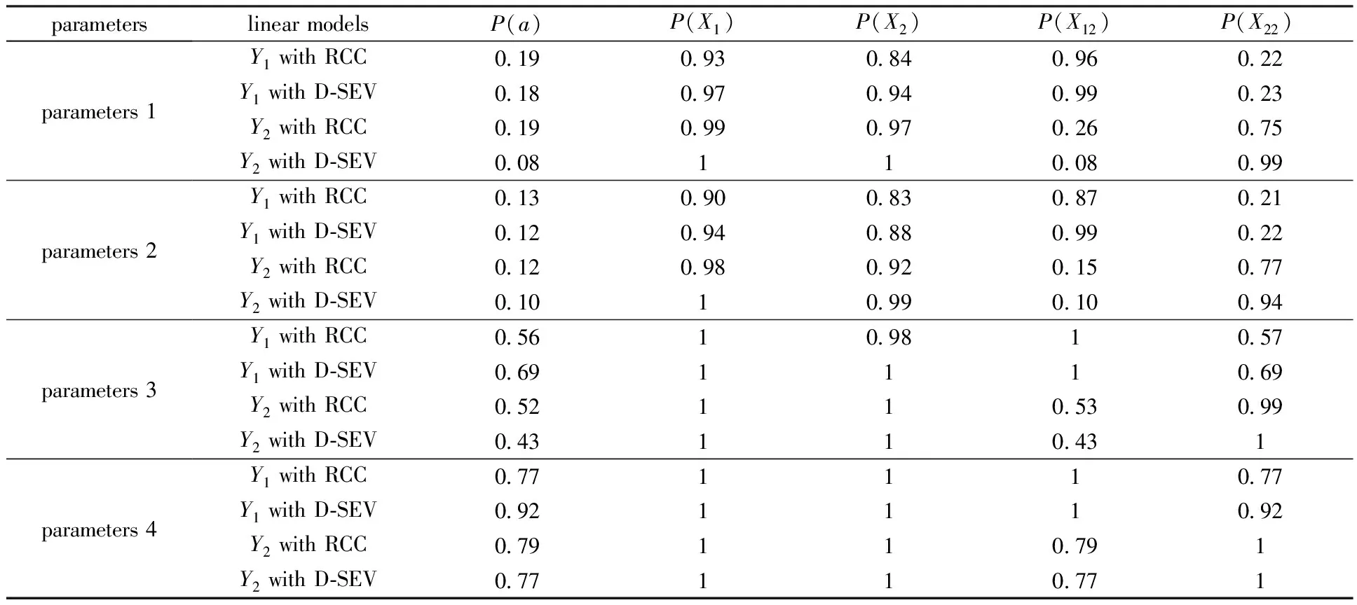
Table 1 Simulation results of P(Xi) and P(a) with RCC and D-SEV

Overall, the performance of robust correlation coefficient achieves advantages on the accuracy of variable selection and computational cost.

4 Empirical analysis

4.1 Empirical data experiment

In this section, we construct the portfolio by robust correlation coefficient with the actual SSE and SZSE stock market data for 2019 and 2020. To calculate the high frequency Sharpe ratio index first, we fixMas 16 andRm,tas Shanghai market index yield. Then the high frequency Sharpe ratio index can be calculated by equation (4). We can see the excellent performance of this index in Fig. 1. After that we establish the portfolio as mentioned in 2.4, we adopt Scroll Window method (DeMiguel et al.[16]) to evaluate the performance of our method. In detail, we denote our sample periods by 20 d asP1,P2…P24,P1stands for the first 20 d. For eacht≥7, we use data inPt-6toPt-1, a total of 120 d to structure the high frequency Sharpe ratio index asYand then pick 30 stocks to constitute the portfolio and hold for 20 d. We choose 30 stocks because we decided to choose 1% of total 3 000 assets. This is what we mentioned above for the purpose of risk diversification. Choosing 20 d as the cycle is similar to the monthly calculation in other articles such as Su and Chen[17], because in a natural month the stock market has about 20 d of opening time. The portfolio is constructed of the stocks selected by equal weighting. In Fig. 2, The portfolio selected by robust correlation coefficient earns 8% more excess annualized return than by D-SEV with the actual SSE and SZSE stock market data for 2019 and 2020. To further compare, another important aspect in portfolio construction is risk, which is emphasized by Markowitz[1]and Sharpe[2]. We calculate Sharpe ratio of each portfolio as the definition of Eq.(1). Sharpe ratio is commonly used to evaluate the risk and return of a portfolio, the portfolio with a high Sharpe ratio will face less risk when the benefits at same level.

The Sharpe ratio of our method is 1.172 while of the D-SEV method is 0.018. The computation time of our method is 17.5 s while of the D-SEV method is 90 067 s.

4.2 Parameter robustness test

Although our method performs much better than D-SEV with fixed parameter setting 30 stocks and 20 d as a period, it is also valuable to check whether our method can achieve similar results in different parameter settings. In this section, we perform the parameter adjustment experiment. From the results obtained in the following figures, we found that our method was relatively robust, and our selection results perform well.

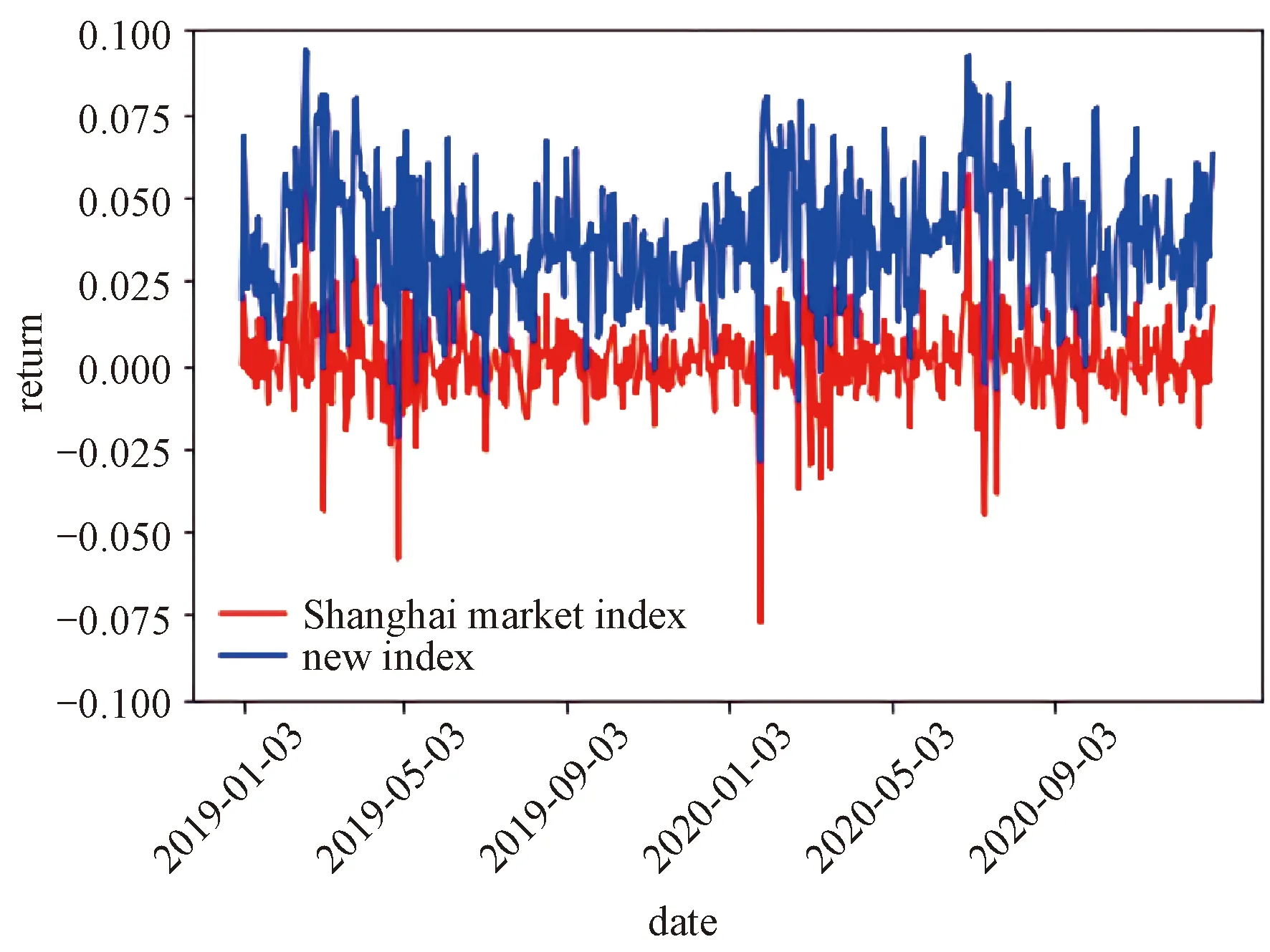
Fig.1 Comparison between returns of high frequency Sharpe ratio index and returns of Shanghai market index in two years

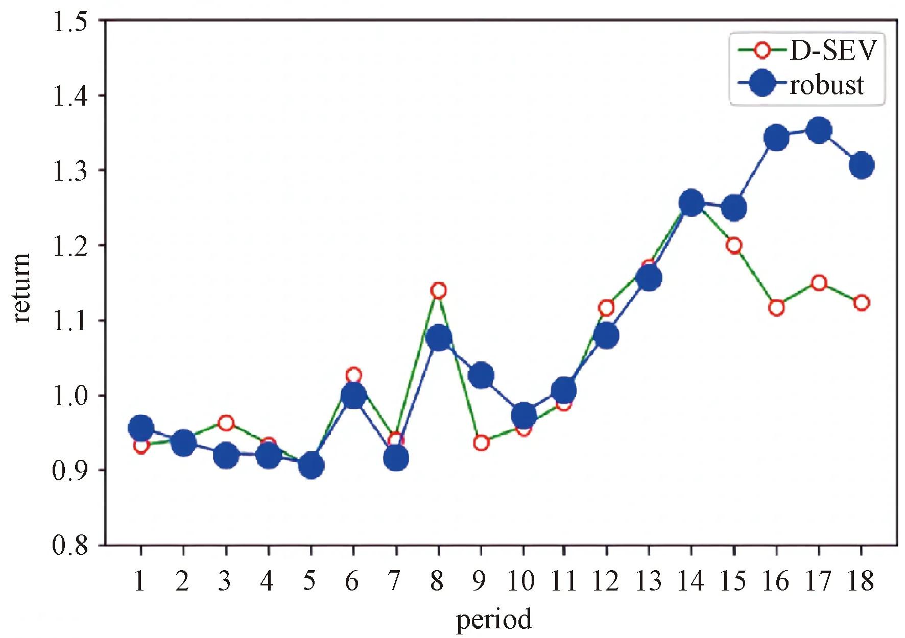
Fig.2 Comparison between returns with our method and returns of D-SEV method in two years under parameters:period=20, stocks=30, time series=120

In Fig. 3(a), we set a period as 18 d with other parameters remain unchanged. The Sharpe ratio in these parameters of our method is 1.47 while of the D-SEV method is 1.11. The computation time in this parameters of our method is 17.9 s while of the D-SEV method is 97 091 s.

In Fig. 3(b), we set a period as 19 days with other parameters remain unchanged. The Sharpe ratio in this parameters of our method is 1.01 while of the D-SEV method is -0.71. The computation time in this parameters of our method is 17.6 s while of the D-SEV method is 89 499 s. In Fig. 3(c), we choose 40 stocks to constitute the portfolio with other parameters remain unchanged. The Sharpe ratio in this parameters of our method is 1.11 while of the D-SEV method is 0.55. In Fig. 3(d), we choose 50 stocks to constitute the portfolio with other parameters remain unchanged. The Sharpe ratio in this parameters of our method is 0.88 while of the D-SEV method is 0.49. In Fig. 3(e), we choose a total of 100 d to structure the high frequency Sharpe ratio index time series asYwith other parameters remain unchanged. The Sharpe ratio in this parameters of our method is 1.91 while of the D-SEV method is 0.41. In Fig. 3(f), we choose a total of 80 d to structure the high frequency Sharpe ratio index time series asYwith other parameters remain unchanged. The Sharpe ratio in this parameters of our method is 1.52 while of the D-SEV method is 0.63.

From the experiments above, the returns of our method performs better than D-SEV under different parameters. Though under some parameters in first 14 periods the returns of the two methods are similar, the Sharpe ratio of our method is obvious higher than that of D-SEV. It indicates that the portfolio of our method has not only more returns but also less risks. Our method itself is very robust in terms of returns and risks. This is due to the robustness of our method as mentioned in section 2.2. Meanwhile, our method has a big advantage over D-SEV in computation time.

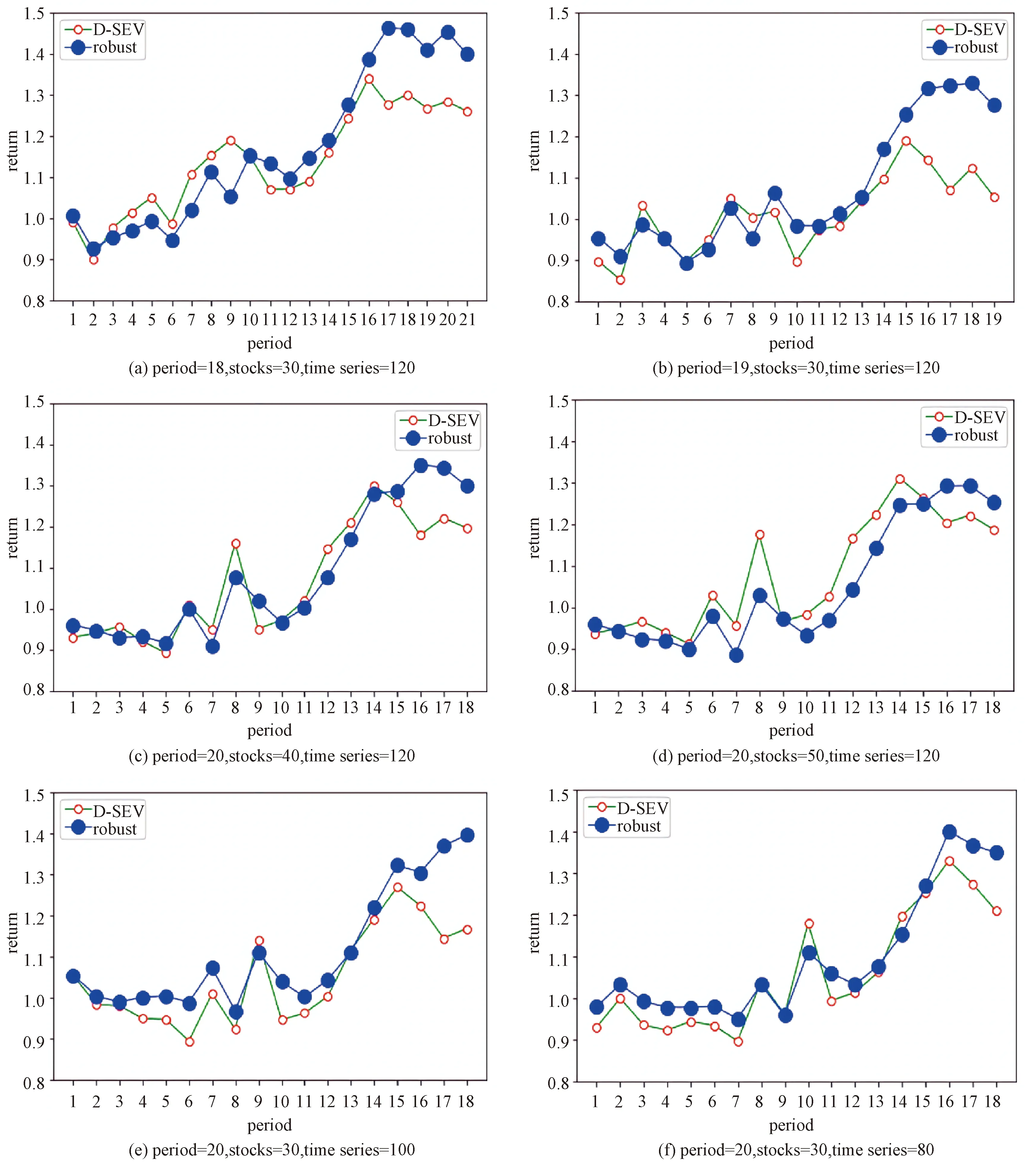
Fig.3 Parameter robustness test

5 Conclusion

In this paper, we filter assets to establish a portfolio based on high frequency Sharpe ratio and the robust correlation coefficient. We are among the first to introduce the robust correlation coefficient in asset selection. The robust correlation coefficient guarantee robustness and less computation cost. These benefits are demonstrated by our simulation and empirical analysis. Our method provides a robust way to construct assets portfolio which generate high return with low risk. Meanwhile, it is relatively easy to implement.