A collaborative assembly for low-voltage electrical apparatuses*#

Huanpei LYU ,Libin ZHANG ,Dapeng TAN‡ ,Fang XU

1College of Mechanical Engineering,Zhejiang University of Technology,Hangzhou 310014,China

2College of Digital Technology and Engineering,Ningbo University of Finance and Economics,Ningbo 315175,China

Abstract: Low-voltage electrical apparatuses (LVEAs) have many workpieces and intricate geometric structures,and the assembly process is rigid and labor-intensive,and has little balance.The assembly process cannot readily adapt to changes in assembly situations.To address these issues,a collaborative assembly is proposed.Based on the requirements of collaborative assembly,a colored Petri net (CPN) model is proposed to analyze the performance of the interaction and self-government of robots in collaborative assembly.Also,an artificial potential field based planning algorithm (AFPA) is presented to realize the assembly planning and dynamic interaction of robots in the collaborative assembly of LVEAs.Then an adaptive quantum genetic algorithm (AQGA) is developed to optimize the assembly process.Lastly,taking a two-pole circuit-breaker controller with leakage protection (TPCLP) as an assembly instance,comparative results show that the collaborative assembly is cost-effective and flexible in LVEA assembly.The distribution of resources can also be optimized in the assembly.The assembly robots can interact dynamically with each other to accommodate changes that may occur in the LVEA assembly.

Key words: Low-voltage electrical apparatus;Collaborative assembly;Artificial potential field based planning;Adaptive quantum genetic algorithm;Dynamic interaction

1 Introduction

Low-voltage electrical apparatuses (LVEAs) are used to achieve the switching,control,protection,detec‐tion,transformation,and adjustment of circuits or non-electric objects (Li DL,2004).LVEAs have wide applications in daily life.Due to their various and complex structures,they are often assembled on a traditional assembly line.Nevertheless,due to varied and rapidly changing requirements,traditional assem‐bly lines cannot satisfy market requirements.These tra‐ditional assembly lines of LVEA are labor-intensive and inflexible,and cannot enable a manufacturer to obtain a dominant position within a fiercely competi‐tive global market (Ge et al.,2021).Many manufac‐turers of LVEAs have emphasized the application of a new assembly method to replace traditional assem‐bly lines.Based on the structural characteristics and usage requirements of LVEAs,there are some require‐ments proposed for LVEA assembly: the assembling resources should be allocated quickly,and the assem‐bling processes should be orderly,stable,and auto‐matic.Additionally,the types of assembled products should be able to be varied.Therefore,it is challeng‐ing to construct a new assembling method for assem‐bling LVEAs.

Nowadays,robot assembly (RA) is extensively applied in product assembly.Compared with traditional assembly lines,RA can achieve 24-h uninterrupted operation with no need for skilled assembly workers.In the assembly of LVEAs,the application of RA could greatly reduce labor costs (Li L et al.,2020;Wang YY et al.,2021).The study of LVEA assembling methods has become much more significant.

Many different applications of RA have been extensively researched by scholars,such as in the methods,planning,and balancing of assembly (Gao et al.,2009).The results have been useful in the study of LVEA assembly.Yu and Yang (2018) proposed a design method for a flexible assembly to achieve realtime adjustment of assembly tasks based on the assem‐bly characteristics of multi-batch small-scale products.Çil et al.(2017) constructed a robotic parallel assem‐bly system and optimized its assembly process using a beam search approach.For the multi-criterion opti‐mization of a multi-product assembly line,Tavakoli (2020) proposed an integer programming model opti‐mized by the hybrid tabu search simulated annealing algorithm (Zheng et al.,2021).For a mixed-model sequencing problem with stochastic processing time in a multi-station assembly line,Li XL et al.(2021) proposed a hybrid particle swarm optimization (PSO) algorithm to deal with the scheduling problem of flexi‐ble assembly systems without intermediate buffers.

In addition to constructing the assembly method and optimizing the assembly planning for RA,it is necessary to optimize the balancing of the complete assembly lines.This is known as the robot assembly line balancing problem (RALBP).In assembly pro‐duction,two main types of assembly balancing prob‐lem occur.The first pertains to minimizing the number of assembly robots within a specific assembly cycle (RALBP-1).The second is related to minimizing the assembly time for a process involving a specific num‐ber of robots (RALBP-2) (Grzechca,2014;Samouei et al.,2016).Regardless of the problem types,the ultimate goal of balanced optimization is to reduce the jobless rate of assembly equipment and improve the efficiency of an entire assembly line.For the balance optimization problem involving robot assembly lines,Rubinovitz et al.(1993) modeled the RALBP-1 problem and applied the best-first search and branch-definition algorithm for optimization.After that,other scholars applied genetic algorithms (GAs),hybrid genetic algo‐rithms (Levitin et al.,2006),and PSO algorithms to optimize the RALBP-2 problem of linear robot assem‐bly lines (Nilakantan et al.,2015;Chen and Tan,2018).The balance optimization problem of a robot assem‐bly line is an extension of the general assembly bal‐ance optimization problem in RA applications (Bay‐bars,1986).Özcan and Toklu (2009) applied a hybrid improved meta-heuristic algorithm to optimize the RALBP-1 problem for simple linear and U-shaped assembly lines.Other researchers proposed planning methods for human–robot collaborative assembly lines (Rizwan et al.,2020;Wang H et al.,2022),and a perfor‐mance evaluation model was established to evaluate the feasibility of multi-resource collaborative assembly systems (Johannsmeier and Haddadin,2017).The pub‐lications mentioned above are summarized in Table S1 (see supplementary materials for Tables S1‒S15).

First,based on the requirements of LVEA assem‐bly,robots require certain communicative functions.The real-time assembly information for each robot needs to be obtained quickly to make a decision for sub‐sequent assembly tasks.The whole assembly line needs to be able to accommodate changes that are needed for making various new products.Second,robots require certain capacities for self-government.When a fault happens in the assembly process,a robot must be able to continue to carry out assembly tasks itself,not dis‐turbed by the fault of other assembly cells.The whole assembly line needs to maintain stability due to the rela‐tive independence of all robots.Third,with a variety of assembly products and an uncertain assembly situ‐ation,the robots need to have dynamic interactions with each other.However,according to Table S1,exist‐ing assembly lines or methods do not satisfy the assem‐bly requirements of LVEAs.Hence,in this paper,we propose a collaborative assembly for LVEA,which will fully satisfy the assembly requirements of LVEAs.The main contributions of this paper are as follows:

1.A collaborative assembly method is proposed for the assembly of LVEAs.

2.An artificial potential field based planning algo‐rithm (AFPA) is proposed to achieve assembly planning and dynamic interaction in the collaborative assembly of LVEAs.

3.An adaptive quantum genetic algorithm (AQGA) is proposed to optimize the assembly processes.

4.A colored Petri net (CPN) model is constructed for the analysis of the collaborative assembly.

The main content of this paper is shown in Fig.S1 (see supplementary materials for Figs.S1–S16).

2 Problem definition

In the assembly of an LVEA,many specific tasks have predetermined precedence relationships and as‐sembly times for each robot.With assembly balance planning,each robot can perform many more tasks in a given time.However,when changes occur in the assembly processes,such as production shifts or robot failures,the balance will be broken.The whole assem‐bly line needs to be adjusted to accommodate the new situation,and the adjustment has a high cost.In the collaborative assembly of an LVEA,the robots can exchange information with each other,and when uncer‐tainty happens,the robots can quickly adjust them‐selves to maintain the stability of the assembly pro‐cesses.For the whole assembly process of an LVEA,the robot assembly is collaborative,and it is neces‐sary to maintain the dynamic interaction of the robots to improve assembly efficiency.In brief,the collabor‐ative assembly of an LVEA has two main challenges: (1) robot interaction and self-government;(2) assem‐bly planning and balance optimization.To solve the problems mentioned above,certain assumptions are made,as follows:

1.Each robot can perform only two kinds of sim‐ple assembling actions.

2.The assembly time of a task is constant and known.The time may vary according to the types of tasks.

3.Each task can be completed by one kind of sim‐ple assembling action.

4.The time consumed in material flow is not con‐sidered in this study.

5.The precedence diagrams are known,and the division of tasks is not allowed.

6.The assembly time of the LVEA is constant.

3 Overview of methodology

This section provides a practical overview with respect to the identification of the collaborative assem‐bly in the assembly of an LVEA.The collaborative assembly processes consist of many necessary basic actions (inserting,putting,rotating,pressing,sticking,and welding) that can be arranged and combined in a particular order to complete the assembly.Each robot can perform two different basic actions.Therefore,during the assembly processes,based on the informa‐tion and characteristics of the LVEA released by the product information database,robots can be scheduled to achieve specific assembly functions according to a specific assembly action sequence.When the product type is changed,the assembly sequence of robots can be quickly reorganized to complete the assembly of the LVEA.The framework of the proposed assembly line is shown in Fig.1.Additionally,for the efficient running of a collaborative assembly line,the collab‐orative assembling methodology is proposed in this section.The architecture of the collaborative method‐ology for LVEA assembly is shown in Fig.S2.It con‐sists of four parts,parts I–IV.Each part has a specific function.Collaborative assembly can be achieved in LVEA assembly with the cooperation of these four parts.

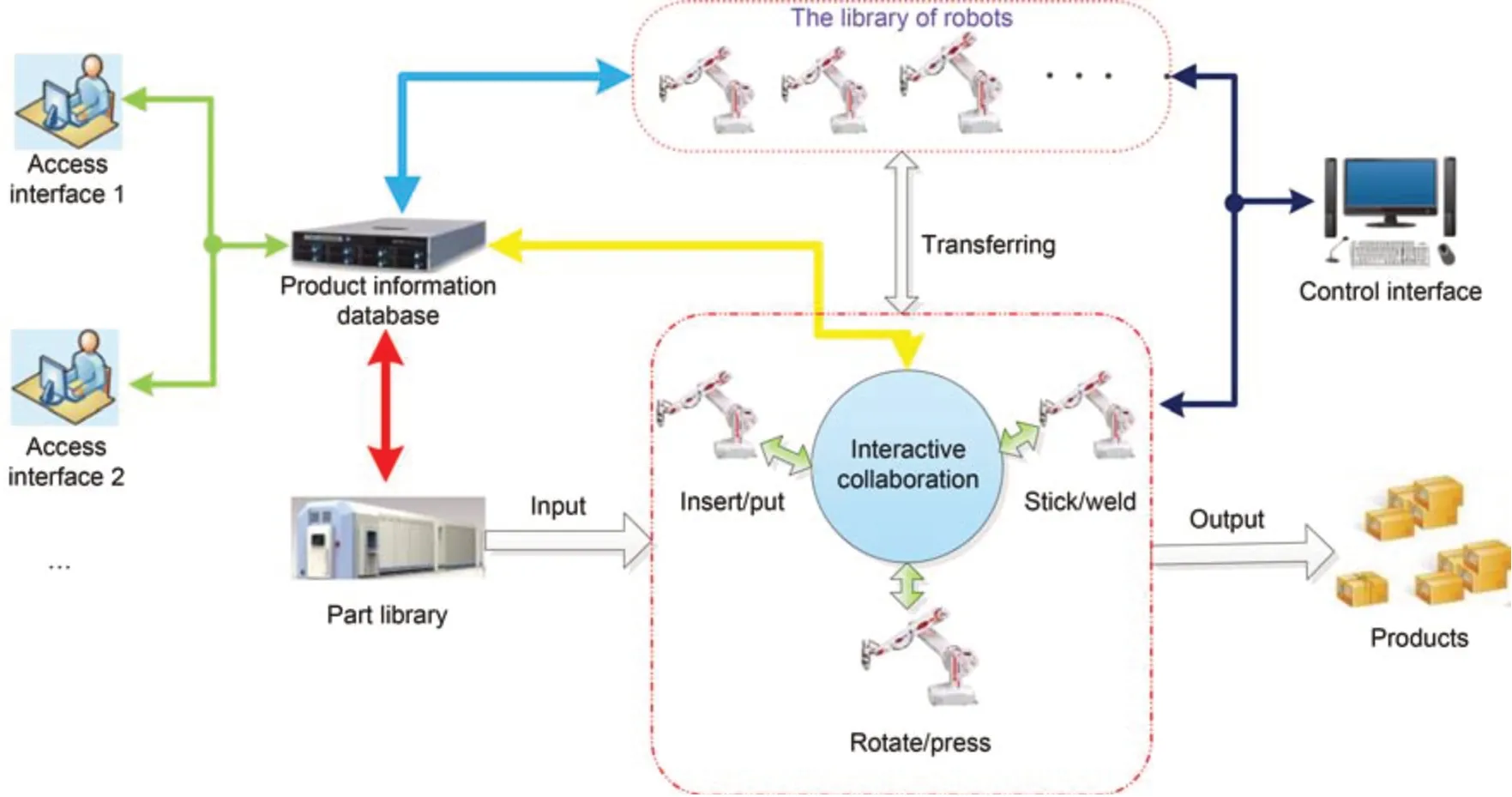
Fig.1 A collaborative assembly

In part I,assembly planning with AFPA is pro‐posed to assign assembly tasks to robots.The robot number and task priority coefficient are obtained.In part II,an AQGA is proposed to optimize the robot number and task priority coefficient (assembly bal‐ance optimization).The distribution of tasks is opti‐mized in this part.Accordingly,the assembly plan‐ning of the collaborative assembly is realized by the combination of parts I and II.In part III,the dynamic interaction based on AFPA is proposed.In this part,the robots can autonomously select tasks based on the priority coefficients of all tasks.The robots can communicate assembly information with each other to maintain dynamic interaction by applying AFPA.In part IV,CPN is applied to construct the collabora‐tive assembly model.The feasibility of the collabora‐tive assembly for LVEA is analyzed with the CPN model.

For the evaluation of the proposed collaborative assembly,LE and SI (Özcan and Toklu,2009;Bat‐taïa and Dolgui,2013) are introduced.As shown in Eqs.(1) and (2),the maximum value of LE is used to reduce the number of robots,and the distribution of the assembly tasks among robots is balanced by reducing SI.Therefore,in part III,LE and SI are applied to evaluate the performance of AFPA.In parts I and II,multi-objective optimization fitness (see Eq.(3)) is introduced to evaluate the performance of AQGA.SI0and LE0are the initial values of SI and LE,respectively.

With dynamic interaction performance,the collab‐orative assembly has good compatibility in the assem‐bly of various LVEAs.Eq.(4) is introduced to evaluate the compatibility of the assembly line.In Eq.(4),it is assumed that there are two types of LVEAs.The first is modelr,and the second is modelp.SrandSpare the numbers of robots used in assembling modelrand modelp,respectively.ELrand ELpare the maximum values of EL when assembling modelrand modelp,respectively.SIrand SIpare the minimum values of SI when assembling modelrand modelp,respectively.WhenSr=Sp,ELr=ELp,SIr=SIp,the value of Cmp is equal to 1,and the assembly line has much better compatibility.where STsis the assembly time of assembly stations,STmaxis the maximum assembly time in all assembly stations,mis the number of assembly stations,andCis the assembly cycle of the product.

4 Artificial potential field based planning algorithm

In the collaborative assembly of an LVEA,each robot has its own tasks.For robots of the same type,con‐fliction may occur when they select the same task.For the tasks with no restriction in the assembly sequence,confliction may occur when the tasks are selected by one robot.Therefore,in the collaborative assembly of LVEA,interactive feedback is necessary between the robots and tasks,and for the flexibility of the col‐laborative assembly,robustness is necessary in the assembly of LVEA.To satisfy these requirements pro‐posed above,an AFPA is proposed in this paper.

The classical artificial potential field (APF) method is a path planning approach to make a robot move from its starting point to a goal (Khatib,1986) while avoiding obstacles on its way.In an APF,an attract‐ing APF which attracts robots is assigned to the des‐tination point,and a repelling APF which repels robots is assigned to the obstacles (Montiel et al.,2015;Tan et al.,2018).Based on the influence of these two combined potentials,the robots can move to their des‐tinations.The definition of APF (Zhang JY and Liu,2007) is listed in Fig.S3.

Based on the theory of APF,AFPA is proposed for the collaborative assembly of LVEA.In the control of AFPA,each task is attracted by the robots,and the dif‐ferent kinds of tasks have different values of the attract‐ing force.According to the value of the attracting force,the assembly tasks can be selected in sequence.

In the collaborative assembly of LVEA,the as‐sembly tasks can be distributed to the robots quickly before assembly,and the robots can interact with each other dynamically during the assembly process.Hence,AFPA has two functions to control the collaborative assembly: (1) distribution of the tasks before assembly;(2) dynamic control of the interaction between robots and tasks.

4.1 Distribution of tasks

In the distribution of the tasks,the main goal is to achieve the scheduling of the robots statically.The sequence of assembly tasks is determined,and the prior‐ity coefficientγiof each task is obtained.It is assumed that in AFPA,ρstiexists between each assembly robot and assembly task (one or more assembly actions):

whereρstiis the static potential distance for taski,ωstiis the static potential of taskiin AFPA,andηstiis the static field charge of taskiin AFPA.

wheremstiis the static quality factor of taskiandtiis the time cost in the completion of taski.

Therefore,the potential field force is calculated as follows:

whereFst-attijis the static potential attractive force of taski,Fst-repijis the static repulsive force generated by taski,andμstjis the class factor.

whereα=1,2,… is the type number of the assembly robot.

ηstiis given as follows:

Therefore,the force of potential field is

According to the math model proposed above,the distribution process of tasks with AFPA is as follows:

1.Initialize each assembly task withFst-attij=0 andFst-repij=0.

2.Analyze and calculate the static potentialωstiand static field chargeηstiof each assembly task in the potential field.

3.Calculate the static potential forces generated by the robots for assembly tasksFst-coij=Fst-attij+Fst-repij.The robot with the largest potential forceFst-co_maxperforms the corresponding assembly tasks.Reset the potential field load of the selected task to 0.

4.Analyze and calculate the static potentialωstiand static field chargeηstiof each assembly task in the potential field again.Recalculate the static situational forcesFst-coijfor unfinished tasks.

5.IfFst-coij=Fst-co_max,perform theithassembly task and reset the static potential and static field load of theithtask to 0;otherwise,continue searching forFst-co_max.

6.Repeat steps 2–5 until the static potential of the final assembly task and the static field load are reset to 0.

In this distribution process,the values ofti,μsti,andmstiare given first,the priority coefficientγiof the tasks is obtained,the scheduling of the assembly robots is achieved,and finally the sequence of tasks is determined.

4.2 Construction of a dynamic interaction pattern based on AFPA in the assembly

After the distribution of assembly tasks with AFPA,each assembly robot acquires assembly tasks correspondingly.If any robot fails,the corresponding tasks will not be completed,which will affect the assembly of the product.Therefore,it is necessary to set up a dynamic interaction pattern between the assem‐bly robots and tasks.Each assembly robot can be fully applied during the assembly process,and the assem‐bly process will not be stalled due to robot failures.In this study,a dynamic interaction pattern based on AFPA is introduced to achieve dynamic,collaborative inter‐action between a robot and a task.The related mathe‐matical model is defined below.

wherenis the number of assembly tasks.Concurrently,the task has a corresponding task excitation factorεiand task guidance factorσi.

The role of the assembly robot in the assembly task has a particular scope;namely,there is a bound‐ary between the assembly robot and the assembly task.Only within this boundary can the robot act on the cor‐responding assembly task.This boundary is defined as the potential field boundary in this study.For each assembly task,the corresponding boundary entry value is given by the potential field boundary Sti:

where Otli−1is the boundary coefficient of the adjacent predecessor taski−1 of taski.When the corresponding assembly taski−1 is completed,Otli−1=1;when taski−1 is not completed,Otli−1∈(0,1).

where Valv is the entrance threshold of the potential field boundary.Only when Sti≥Valv,can assembly tasks pass through potential field boundaries.

When assembly tasks cross the potential field boundary,they are subject to the dynamic forcesFrtijof robotjon taski:

where Mrjis the mass property of robotj,drijis the dy‐namic potential distance between robotjand taski,andψjis the state parameter of assembly robotj.ψjsatisfies

Additionally,Δjis the type factor of assembly robotj.If the assembly tasks belong to assembly robotj,thenΔj=1;otherwise,Δj=0.

They were pawing the ground in their impatience52 to start, and the merchant was forced to bid Beauty a hasty farewell; and as soon as he was mounted he went off at such a pace that she lost sight of him in an instant

Whenψj=1,the task is attracted byFrtij;whenψj=−1,the task is repelled byFrtijfor the case of AFPA.

According to the math model proposed above,the dynamic interaction pattern with AFPA in assembly is as follows:

1.Initialize each assembly task.The correspond‐ing boundary coefficient Otliranges in (0,1).Accord‐ing to the priority coefficientγi,calculate the stimu‐lus factorεiand its boundary attributes for each task in the initial state.

2.Each assembly robot issues an assembly instruc‐tionψj=1.The potential field boundary is opened,and the threshold of the boundary entry is taken as Valv=min(λ1,λ2,…,λn).Calculate the boundary entry value Stifor each assembly task.

3.Determine whether Stiof each task is greater than the threshold of the boundary entrance.If Stiis higher than Valv,the corresponding taskienters the potential field boundary.

4.Each assembly robot attracts the task in the po‐tential field.The potential field forceFrtijis calculated.The robot and the assembly task are matched in order according to the magnitude of the potential force.When the robot obtains the corresponding assembly task,the state parameter of the assembly robotψj=−1.

5.When taskiis completed,its corresponding boundary coefficient Otliis set to 1.The initial adja‐cent predecessor task boundary coefficient Otli−1is reset to its original value,in (0,1).The state parameter of the assembly robot isψj=1.

6.Return to step 3 and perform the calculation again until all assembly tasks are completed.

In this process,the priority coefficientγiof the tasks is given first,and the dynamic interaction pat‐tern is established last.

5 AQGA algorithm

In the collaborative assembly,with the different assembly sequences of each assembly task,the re‐quired assembly time and the number of assembly robots vary.According to the structure of LVEA,it is necessary to balance and optimize the number of robots.In this study,the assembly time for LVEA is selected.Then,the number of assembly robots (that is,the RALBP-1 assembly balance problem) needs to be optimized.This is a non-deterministic polyno‐mial (NP-hard) problem.Many previous studies have proven that evolutionary algorithms are effective in solving NP-hard problems (Li L et al.,2021).To this end,an AQGA is introduced.

The quantum genetic algorithm (QGA) is a proba‐bilistic search optimization algorithm based on the com‐bination of quantum computing theory and evolution‐ary algorithms.In QGA,the chromosomes are repre‐sented by qubit encoding,and the evolutionary search is completed by quantum gate action and a quantum gate update (Yang et al.,2003).Since QGA has a small population size that does not affect the per‐formance of the algorithm,QGA has a high conver‐gence speed and strong global searchability.Hence,it has attracted attention from researchers worldwide.In this study,a QGA and an AFPA are combined to achieve collaborative assembly control.The specific mathematical model of AQGA can be given as follows.

In QGA,the smallest information unit is repre‐sented by a qubit.The state of a qubit can be expressed as follows:

whereαjandβjmeet the following conditions:

Concurrently,a pair of complex numbers (αj,βj) is known as a probability bit of a qubit,expressed as [αj,βj]T.

In the real number encoded QGA,the probability amplitude is directly applied for encoding.The spe‐cific encoding scheme is shown in Eq.(22):

In Eq.(22),θij=2π·rand,rand is a random num‐ber in (0,1),i=1,2,…,m,j=1,2,…,n,mis the size of the population,andnis the number of quanta.

Assuming that the optimization variable solution range is [Xmin,Xmax],the observed state of the quan‐tum superposition is solved with

wherei=1,2,…,m,j=1,2,…,n.

In the quantum phase rotation update,a method based on the gradient of the objective function is pro‐posed (Li SY and Li,2006) for controlling the rota‐tion phase step size,as shown in Eq.(24).Accord‐ingly,we introduce an adaptive function based on maxi‐mum fluctuation.The adaptive function can further control the step size search accuracy to avoid local optima.

where sign(Comp) is the phase turning function,Comp=det(ω0,ω1),ω0=[α0,β0]Tis the probability magnitude of the optimal solution for the current search,andω1=[α1,β1]Tis the probability amplitude of the current solution.

In Eq.(25),kis the adaptive coefficient,and avg is the mean fluctuation function:

whereδ1is the absolute value of the difference between the average Fitness value and the minimum Fitness value,andδ2is the absolute difference in the mean Fitness between the two generations.Accordingly,the improved quantum phase rotation update formula is

whereθis the updated quantum phase andθ0is the original quantum phase.The specific implementation process of AQGA is initiated as follows:

1.Initialize the population.The population sizen,number of qubitsm,and probability of quantum mutationPmare given.PopulationQcontains many individuals,i.e.,Q={q1,q2,…,qn},whereqj(j=1,2,…,n) is thejthindividual,andnis the number of individuals in the population.A specific description is as shown in Eq.(22).

2.Construct the observed state of quantum super‐position stateQchiaccording to the probability ampli‐tude of each body inQi,whereQchi={qchi1,qchi2,…,qchin},andqchij(j=1,2,…,n) is the observation state of thejthindividual.A specific description is as shown in Eq.(22).In QGA,the process of constructing the obser‐vation stateQchifrom the probability amplitudeQincludes a decoding process,and the actual values of the optimization parameters are obtained after decoding.

3.Calculate the Fitness of the observed state and the optimal value.

4.Retain the best individual and determine whether the termination condition is met.If the condition is satisfied,the algorithm is terminated;if not,go to the next step.

5.Calculate the phase of the quantum-revolving gate according to Eq.(23),and apply the updated quan‐tum phase in Eq.(23) to act on the probability ampli‐tudes of all individuals in the population.

6.Perform quantum phase mutation operations to generate a new population,and updateQchi.

7.Perform fitness evaluation calculations and cal‐culate the optimal solution after phase update mutation.

8.Compare the previous optimal solutions with the optimal solutions after phase update mutation.If the optimal solution is degraded,the previous optimal solution is retrieved.If the optimal solution evolves,the optimal solution is replaced.

9.Increase the evolution generation and return to step 2.The calculation will not be completed until the minimum robot number is obtained.

6 Construction of the collaborative assembly model based on CPN

To analyze the performance of the proposed col‐laborative assembly of an LVEA,the assembly model must be constructed.Since the collaborative assembly process of an LVEA is characterized by parallel,asyn‐chronous,event-driven,deadlock,and conflict elements (Xie,2006;Zeng et al.,2014),the entire assembly is a discrete event dynamic system (Charbonnier et al.,1999;Zelenka,2010;Wang JX et al.,2023).The pri‐mary modeling methods of this type of system are classified as follows (New,1994;André et al.,2016;Pan et al.,2020;Zhang K et al.,2022): (1) graphic–analytic hybrid modeling theory,e.g.,queuing theory,Markov chains,and Petri net modeling theory,(2) mod‐eling theory based on artificial intelligence,e.g.,agent systems and Holon whole subsystems,(3) granularity calculation analysis theory,and (4) modeling theory based on matrix operation,among others.

Based on the assembly characteristics of LVEA,CPN modeling theory is applied to establish the assem‐bly model in this study.This model reflects the sequence,parallel,synchronous,and asynchronous characteris‐tics of discrete events,and colored tokens are used to colorize different assembly tasks and instructions.The CPN theory is based on the place/transition Petri nets (Desel and Reisig,1998),which are the most promi‐nent and best studied class of Petri nets.The formal definition of CPN (Jensen,1990) is given in Fig.S4.

Accordingly,based on the overall design idea for the collaborative assembly,and the CPN modeling the‐ory,the CPN collaborative assembly model comprises mainly the place setP,transition setT,and arc setA.Based on the CPN modeling theory,the corresponding place,transition,and arc set for each unit in the collab‐orative assembly are designed with the software pack‐age CPN Tools (v.4.0.1).The places and transitions in the assembly model are defined in Figs.S5 and S6,respectively.

7 Simulation analysis

To verify the effectiveness of the collaborative assembly of LVEA,in this work we adopted a twopole circuit-breaker controller with leakage protection (TPCLP),which is one kind of LVEA,as an example for simulation analysis.The processor of the computer used in this simulation was an Intel®CoreTMi5-6200U CPU with 4 GB memory.

During the assembly of TPCLP,six assembly functions were required: inserting,putting,rotating,pressing,sticking,and welding.After disassembling and analyzing the product,in the assembly of this product,45 assembly tasks had to be performed,each of which was represented by a corresponding letter.In collab‐orative assembly,each robot can perform only two assembly functions,so three robots with different func‐tions were needed to complete the assembly.The corre‐sponding relationship between the robot and the as‐sembly task is shown in Table S2,whereRprepre‐sents an assembly robot with insertion and putting functions,Rsrepresents a robot with rotation and pres‐sure functions,andRwrepresents an assembly robot with welding and adhesion functions.The constraint relationship between tasks is shown in Fig.S7,in which the number next to each task name mentioned above is the time consumed in completing the assem‐bly task.

During the collaborative assembly of TPCLP,some requirements had to be met: (1) In the assem‐bly process,it was necessary to satisfy the assembly constraint relationship between the various tasks shown in Fig.S7.(2) During the assembly process,assembly conflicts between robots and assembly tasks had to be avoided.(3) Scheduling too many robots had to be avoided since this can result in a waste of resources.Therefore,in a given assembly cycle,the total number of robots employed had to be as low as possible.

To verify the feasibility of the collaborative assem‐bly proposed above,some functions were needed in the simulation.First,the CPN model of collabora‐tive assembly was established to analyze the interac‐tion and self-government of the robots.Second,some evaluation parameters,such as LE,SI,and Cmp,were calculated to analyze the assembly planning and dy‐namic interaction of the collaborative assembly.The main work of this part was as follows:

7.1 CPN model construction of the TPCLP assembly

According to the proposed collaborative assem‐bly,taking TPCLP as an example,the specific assem‐bly of the cooperative assembly process was analyzed using CPN Tools.The entire assembly method model primarily included a task data unit,an assembly robot unit,an information-processing unit,and a product task detection unit.

Additionally,some parameters needed to be set before the assembly analysis.Based on the assembly balance analysis of AQGA,the number of robots varied with the value of the assembly cycle,which can be found in Table S3.

In this assembly analysis,the assembly cycle was set to 90 time units.Accordingly,the number of robots was five,including twoRp-type robots,twoRs-type robots,and oneRw-type robot.The number of assem‐bly products to be completed was 10.With the com‐bination of the assembly units,the CPN collaborative assembly model is as shown in Fig.2.

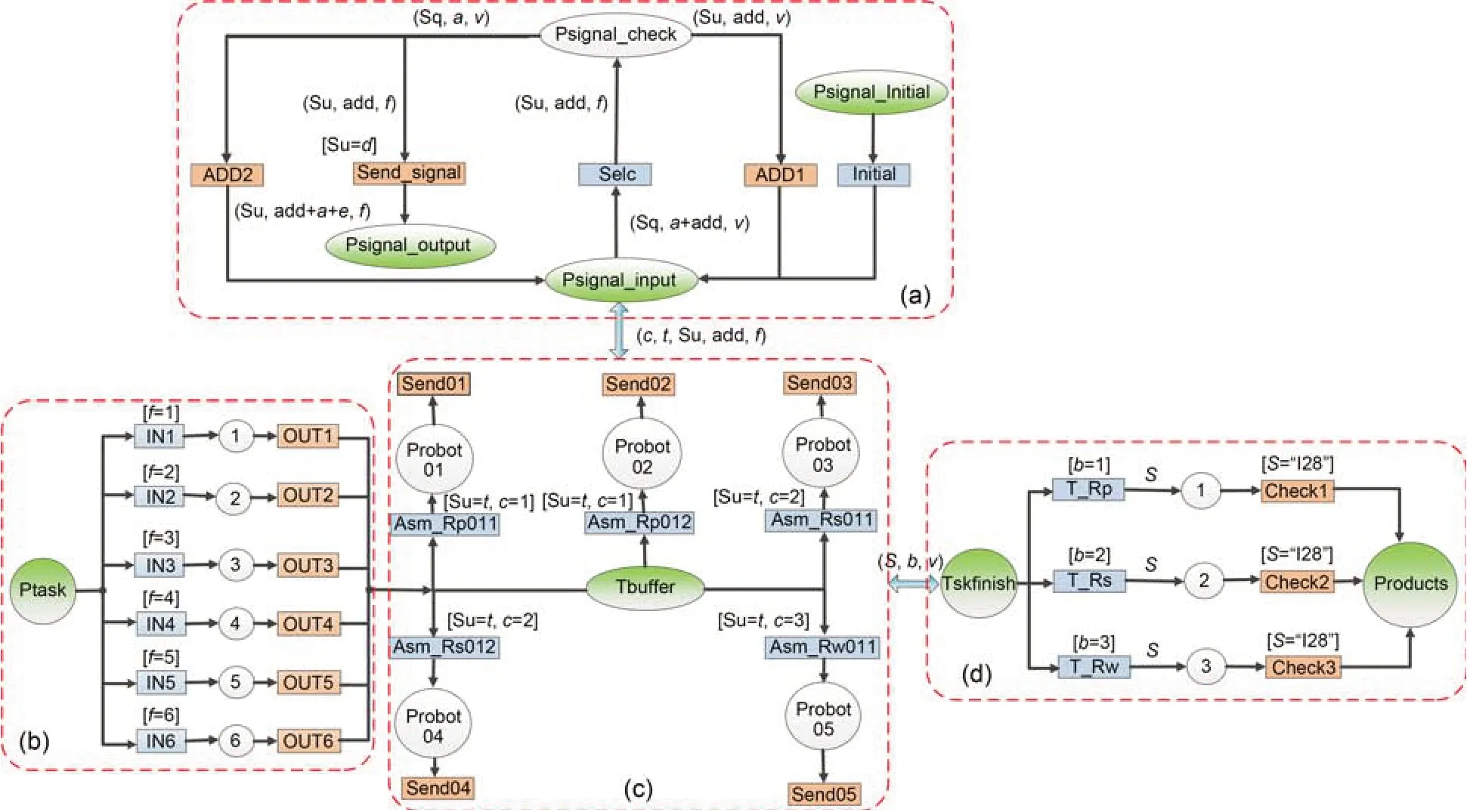
Fig.2 CPN collaborative assembly model: (a) product and task detection unit;(b) task data unit;(c) assembly robot unit;(d) information processing unit

Based on the CPN collaborative assembly model,the simulation monitoring unit Monitor in CPN Tools was used to analyze the interaction and self-government of the robots.By applying the “Count Transition” func‐tion in the simulation control unit Monitor,some changes were observed in the system (Asm_Rp011,Asm_ Rp012,Asm_Rs011,Asm_Rs012,Asm_Rw011,T_Rp,T_Rs,and T_Rw),and the number of completed tasks of the five robots was analyzed.The results are listed in Table S4.By the monitoring of transitions T_ Rp,T_Rs,and T_Rw (Fig.2),the number of completed assembly tasks in the assembly process was detected.Overall,330 inserting/putting tasks,180 spinning/pressing tasks,and 210 welding/sticking tasks were detected.According to the number of tasks obtained by each assembly robot,for the same assembly tasks,the number of tasks for the assembly robots was similar,and each robot maintained good communication to balance the task distribution.Accordingly,as long as the same type of assembly robot operated normally,the failure of some robots would not affect the entire product assembly process.Hence,the robots had a good capability of self-government in the collaborative assem‐bly of LVEA.

The randomness of the distribution process of the tasks should be considered during the assembly.In the multi-batch simulation analysis,three confi‐dence intervals of 90%,95%,and 99% were set to estimate the probability of the assembly tasks being completed by the robots.As shown in Fig.S8,the av‐erage number of assembly tasks performed by each robot was obtained from 10 consecutive simulation analyses.In Fig.S8,the abscissa is a given confidence interval value,and the ordinate is the number of assem‐bly tasks to be performed by each assembly robot.When the confidence interval was 99%,the number of tasks included increased,but they all fluctuated substantially within a stable interval.In Fig.S9,the selected confidence interval was 95%,and the numbers of simulation batches were 5,10,15,20,and 25.Accord‐ing to the confidence curve,during the operation of the assembly system,the number of tasks was stabilized.The number of assembly tasks among robots of the same type also tended to be the same.Therefore,it was found that the robots had good interactivity to main‐tain the stability of the collaborative assembly.

7.2 Analysis of AFPA and AQGA in collaborative assembly

In the collaborative assembly of TPCLP,AFPA and AQGA were applied to control the assembly pro‐cess.Before TPCLP assembly,the number of robots and the assembly planning were optimized.During the TPCLP assembly,the assembly processes were in a dynamic balance to maintain the effectiveness and sta‐bility of the assembly.In the simulation,we analyzed the effectiveness of AQGA applied in the optimiza‐tion of the assembly balance by comparison with other algorithms.AFPA was also analyzed to verify its per‐formance for assembly planning and dynamic inter‐action by comparison with some traditional assembly methods.The details of the simulation analysis pro‐cesses were as follows:

First,the performance of AQGA was analyzed by introducing typical genetic algorithms,including GA,simulated annealing genetic algorithm (GASA) (Baykasoglu,2006;Ren et al.,2015),QGA (Yang et al.,2003),and objective function gradient based quantum genetic algorithm (RQGA) (Li SY and Li,2006),and optimization comparisons were carried out.

In the application of typical genetic algorithms,some critical parameters needed to be set,such as the population size,individual variable dimension,genetic generation,crossover probability,and mutation rate.Based on previous research on GA (Deb,1998;Ji et al.,2012),the critical parameter value range was as shown in Table S5.If the parameter values were not in the given range,it was difficult to obtain the opti‐mization results.According to the number of tasks,the individual variable dimension was 45.According to the analysis,the quantum rotation angle ranged from 0.01 to 0.5.When the value was smaller than 0.01,the calculation burden was increased.However,if the value was larger than 0.5,the optimization results were missed.The relevant parameters of the compared algo‐rithms were set as shown in Fig.S10.

In the comparative analysis of the algorithms,AQGA was compared with commonly used algorithms GA,GASA,RQGA,and QGA based on a combination with AFPA.In this comparison,according to Table S6,the theoretical assembly cycleCtof TPCLP was set to 70,90,110,130,and 150 time units.The target values of the analysis and comparison were Fitness,LE,SI,andS.The specific analysis results were shown in Fig.3 whenCtwas set to 90 time units.The results showed that the AQGA algorithm proposed in this paper had better optimization performance.This algorithm ex‐hibited better convergence performance than the com‐pared algorithms GA,GASA,RQGA,and QGA,and it can rapidly converge within a small number of itera‐tions without being limited to a local optimum.The detailed results of the comparison of the algorithms at differentCt’s are shown in Table S6.We found that through AQGA optimization,the Fitness,LE,SI,Svalues obtained were better than those of the com‐pared algorithms.These results were all better than the optimal values provided by several other algo‐rithms.As shown in Fig.S11,AQGA was better than the compared algorithms in the optimization of the robot number.For the different numbers of assembly cycles,AQGA could calculate the minimum robot number quickly.Hence,AQGA can improve the effec‐tiveness of assembly balancing in the collaborative assembly.

Fig.3 Comparative analysis of a combination of AFPAs with different optimization algorithms: (a) robot number;(b) SI;(c) LE;(d) Fitness

To analyze the performance of AQGA more deeply,a non-parametric statistical test was applied.Twenty samples were selected.The statistical data of the different algorithms are listed in Table S7.The descriptive sta‐tistics and ranks of the robot number (RBN),SI,LE,and Fitness are listed in Tables S8 and S9,respectively.By analysis of Mean,Std.,Min.,Max.,and mean ranks,we can find that the values (RBN,SI,LE,and Fitness) obtained by AQGA were better than those of other algo‐rithms.From Table S10,we can also find that the values ofpwere all smaller than 0.05,so the sampling data obtained from the algorithms AQGA,GA,GASA,QGA,and RQGA were significantly different.

Then,the performance of assembly planning opti‐mization and dynamic interaction of AFPA was ana‐lyzed.The simple straight assembly line (ST_line),twosided assembly line (TS_line),and U-shaped assem‐bly line (U_line) were compared with the collaborative assembly to verify the good performance of AFPA.Fig.4 shows the assembly resource allocation and optimization performance of the collaborative assem‐bly for AFPA and AQGA.Assembly cycles of 90 and 150 time units were selected for comparison and anal‐ysis,the Fitness values of various assembly methods were compared,and the comparison of LE,SI,and RBN were as listed in Figs.S12–S14.It was assumed that during the assembly processes an assembly robot could perform only two assembly actions (such as spinning/pressing,inserting/putting,and sticking/weld‐ing).Therefore,in the basic assembly line (ST_line,TS_line,and U_line),at least three different kinds of robots were required in each assembly station.However,in the collaborative assembly,each assembly station had only one kind of assembly robot.Hence,from Fig.4 and Figs.S12–S14,it can be found that for dif‐ferent assembly cycles,the collaborative assembly had excellent assembly planning optimization and dynamic interaction performance compared with several other basic assembly lines.AFPA significantly improved the utilization efficiency of each robot and optimized the assembly resource distribution.Furthermore,for the same assembly cycle,the collaborative assembly was able to reduce the number of assembly robots to reduce assembly cost.

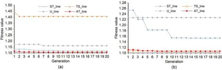
Fig.4 Fitness values of various assembly methods for different assembly cycles: (a) 90 time units;(b) 150 time units

To analyze the performance of AT_line more deeply,a non-parametric statistical test was applied to analyze the performance of AT_line,ST_line,TS_line,and U_line.In this analysis,16 samples were selected.The statistical data,descriptive statistics,and ranks of different assembly lines in terms of RBN,SI,LE,and Fitness are listed in Tables S11–S13.By analysis of Mean,Std.,Min.,Max.,and mean ranks listed in the supplemental materials,we found that the values of RBN,SI,LE,and Fitness obtained by AT_line were better than those of other algorithms.From Table S14,we can also find that the values ofpwere all smaller than 0.05,so the sampling data obtained from assembly lines AT_line,ST_line,TS_line,and U_line were sig‐nificantly different.

To analyze the dynamic interaction performance of AFPA,the values of LE,SI,S,Ct,andCr(actual assembly cycle of the product) were analyzed for com‐parison with the values obtained before dynamic inter‐action,and the compatibility assembly of various prod‐ucts was introduced to analyze the performance of dynamic interaction.

In this simulation different assembly cycles of 70,90,120,and 150 time units were set to analyze changes in the values of LE,SI,andCr,compared with the values obtained before the dynamic interaction of AFPA.The results are shown in Table 1 and Fig.S15.Comparative analysis showed that,through the optimization of the dynamic assembly process with AFPA,the assembly collaboration between the assembly robots was greatly improved and the robots were fully used in the assembly process.Additionally,the algorithm can reduce the assembly time and improve the assembly efficiency.Under the control of the optimization of the dynamic assembly process with AFPA,the product assembly pro‐cess was rendered relatively stable.The values of LE,SI,andCrremained essentially unchanged or fluctuated within a fixed range of values for different cycles.

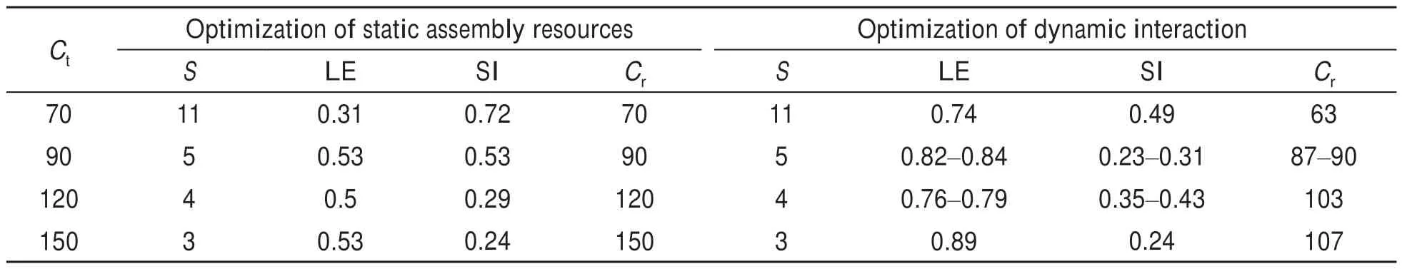
Table 1 Effectiveness of dynamic balance with AFPA

During the assembly of TPCLP,cooperative assem‐bly was achieved by comprehensively applying AFPA and AQGA.Table S15 shows that compared with sev‐eral existing assembly lines,for the different assembly cycles,the collaborative assembly was able to achieve a dynamic interaction between robots with fewer robots,so it could improve the assembly efficiency and reduce the assembly cost.

To analyze the compatibility of the collaborative assembly,another kind of TPCLP,called type 2,was in‐troduced in the simulation (the first kind of TPCLP dis‐cussed above is called type 1).Compared to the assem‐bly of type 1,type 2 had the same assembly number but different kinds of assembly tasks,as shown in Fig.S16.

In the simulation,the collaborative assembly line AT_line was compared with the existing traditional assembly lines in terms of compatibility of the assem‐bly process.The results are shown in Fig.5.

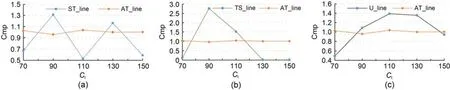
Fig.5 Cmp comparison among different assembly methods: (a) ST_line vs.AT_line;(b) TS_line vs.AT_line;(c) U_line vs.AT_line

According to Fig.5,in the different assembly cycles,the Cmp of the basic assembly methods (ST_ line,TS_line,and U_line) was much larger or smaller than 1.The most significant value was 2.767,and the smallest value was 0.119.However,the Cmp of AT_line was close to 1.The most substantial value was 1.038,and the smallest value was 0.958.Hence,with the dynamic interaction of AFPA,the collaborative assem‐bly line had better compatibility.

8 Conclusions

In this paper,we propose the collaborative assem‐bly of LVEAs.Three objectives were considered: (1) self-government of robots;(2) assembly balance of the collaborative assembly;(3) assembly planning and dynamic interaction of the collaborative assembly.The results are summarized as follows:

1.Through the construction of the CPN collab‐orative assembly model,the self-government of robots was analyzed in the collaborative assembly.As shown in Figs.S8 and S9,with the different confidence inter‐vals (90%,95%,and 99%),all of the assembly robots completed the tasks with a relatively stable number.At five different numbers of simulation batches,each robot completed the tasks with a relatively stable number.Hence,the robots had good performance to avoid assembly confliction in the collaborative assem‐bly.We also found that when one robot was in fault,the assembly process was not interrupted.The robot had good self-government ability to improve the pas‐sive fault tolerance of the assembly process.

2.AQGA applied to balance the collaborative assembly had better convergence performance than the compared algorithms GA,GASA,RQGA,and QGA.Furthermore,with the optimization of AQGA,the Fit‐ness,LE,SI,andSvalues obtained were better than those optimized with the compared algorithms.Hence,AQGA had better performance in collaborative assem‐bly balance.

3.AFPA was proposed to perform assembly plan‐ning and dynamic interaction of the collaborative assembly.Figs.S11–S14 showed that in the applica‐tion of AFPA,the collaborative assembly method could achieve assembly planning and dynamic interaction in the LVEA assembly.Furthermore,compared with the traditional assembly line,the collaborative assembly method achieved better LE,SI,S,and Cmp.

Thus,we can conclude that collaborative assem‐bly is effective in the assembly of LVEAs.

Considering an actual assembly situation,how‐ever,there are two research directions for LVEA col‐laborative assembly.First,the collaborative assembly has passive fault tolerance,but when the assembly pro‐cess is interrupted by multiple faults,the efficiency of LVEA assembly will be affected.Therefore,the active fault tolerance of the collaborative assembly needs to be studied.Second,in LVEA collaborative assembly,the control of assembly robots is distributed.There‐fore,the distributed interactive communication method needs to be researched.

Contributors

Huanpei LYU,Libin ZHANG,and Dapeng TAN proposed the idea.All the authors designed the research.Huanpei LYU drafted the paper.Libin ZHANG,Dapeng TAN,and Fang XU revised and finalized the paper.

Compliance with ethics guidelines

Huanpei LYU,Libin ZHANG,Dapeng TAN,and Fang XU declare that they have no conflict of interest.

Data availability

The data that support the findings of this study are available within the article and its supplementary materials.

List of supplementary materials

Fig.S1 Main content of this paper

Fig.S2 Architecture of the collaborative assembly methodology

Fig.S3 Definition of the artificial potential field (APF)

Fig.S4 Formal definition of the colored Petri net (CPN)

Fig.S5 Setting of places in the CPN collaborative assembly model

Fig.S6 Setting of model transitions in the CPN collaborative assembly model

Fig.S7 Relationship between the tasks required for a TPCLP

Fig.S8 Average number of assembly tasks of the assembly robots for different confidence intervals

Fig.S9 Number of assembly tasks for each assembly robot for different numbers of simulation batches

Fig.S10 Setting of relevant parameters of the compared algorithms

Fig.S11 Comparison of the number of robots required for the different algorithms

Fig.S12 LE values of each assembly mode for different as‐sembly cycles

Fig.S13 SI values of each assembly mode for different assem‐bly cycles

Fig.S14 Number of robots required for each assembly mode for different assembly cycles

Fig.S15 Analysis of the robot assembly performance with dynamic balance of AFPA

Fig.S16 Relationship between the assembly tasks required for type 2

Table S1 Studies of assembly line construction and balance optimization

Table S2 Assembly tasks corresponding to each assembly robot

Table S3 Relationship between the assembly cycle and the robot number

Table S4 Number of assembly tasks for each type of robot

Table S5 Value range of the critical parameters

Table S6 Comparison of optimal target values for each algorithm

Table S7 Statistical data of different algorithms

Table S8 Descriptive statistics of different algorithms

Table S9 Ranks for different algorithms

Table S10 Friedman test statistics of different algorithms

Table S11 Statistical data of different assembly lines

Table S12 Descriptive statistics of different assembly lines

Table S13 Ranks of different assembly lines

Table S14 Friedman test statistics of different assembly lines

Table S15 Comparison between the collaborative assembly and basic assembly lines