Deacy estimates of solutions to two dimensional Schrödinger systems with quadratic dissipative nonlinearities

TANG Shuqi,LI Chunhua

(College of Science,Yanbian University,Yanji 133002,China)

Abstract：The Cauchy problem for systems of two dimensional Schrödinger equations with quadratic dissipative nonlinearities is considered.In the case of the mass resonance,the existence of global solutions to the nonlinear Schrödinger systems with small initial data is discussed and time decay estimates of global solutions are derived.

Keywords：systems of Schrödinger equations;quadratic dissipative nonlinearities;time decay estimates of solutions;mass resonance conditions

0 Introduction

The following Cauchy problem for the nonlinear Schrödinger system is considered

(1)

The study of the Cauchy problem of nonlinear Schrödinger systems is widely used in nonlinear optics.The nonlinear Schrödinger systems with quadratic nonlinearities in two space dimensions are interesting mathematical problems,since they are regarded as the borderline between short-range and long-range interactions.Therefore,the time decay estimates of the nonlinear Schrödinger systems are one of the research highlights.

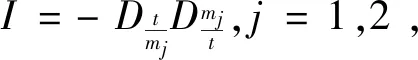
We assume that the masses of particles in the Cauchy problem (1) satisfy the mass resonance condition (H1)2m1=m2.If the condition (H1) holds,then the Cauchy problem (1) meets the following gauge condition

Gj(v1,v2)=eimjθGj(e-im1θv1,e-im2θv2),j=1,2

for anyθ∈.Ifλj=0 forj=1,2 in the system (1),then the system (1) becomes

(2)

(3)

for small initial dataφj∈Hγ,0(2)∩H0,γ(2) with 1<γ<2,wheremjis a mass of a particle,F3(v1,v2,v3)=μ3v1v2,λj,μj∈{0} andφj(x) is a prescribed-valued function on2forj=1,2,3.Since the nonlinearityλj|vj|vjof the system (3) is not included in the system (2),in reference [9] the Cauchy problem (3) is investigated by improving the method of reference [1] .Time decay of solutions

A generalization of the Cauchy problem (2)

(4)

and the time decay estimates

‖v‖L∞(2)≤Ct-1ε

fort≥1.

(5)

Under the assumption that Imλj≤0 forj=1,2,by the system (5),we obtain

1 Main results

Theorem1Suppose that the assumptions of Proposition 1 are satisfied.Letvbe the solution to the Cauchy problem (1) whose existence is guaranteed by Proposition 1.If Imλj<0 forj=1,2,then we have

(6)

for allt≥0.

Remark1We consider a generalization of the Cauchy problem (1)

(7)

whereGj(v1,…,vl)=λj|vj|vj+Fj(v1,…,vl),λj∈{0},mjis a mass of a particle and quadratic nonlinearityFjhas the form

(8)

Gj(v1,…,vl)=eimjθGj(e-im1θv1,…,e-imlθvl)

(9)

and

Imλj<0

(10)

2 Preliminaries

In this section,we give some results as preliminaries.In what follows,we use the same notations both for the vector function spaces and the scalar ones.For anypwith 1≤p≤∞,Lp(2)denotes the usual Lebesgue space with theif 1≤p<∞ andFor anym,s∈,weighted Sobolev spaceHm,s(2) is defined by

Hm,s(2)={f=(f1,f2)∈L2(<∞}

where the Sobolev norm is defined as

forj=1,2.We denote various positive constants by the same letterC.

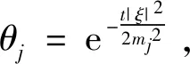
We define the dilation operator by

and

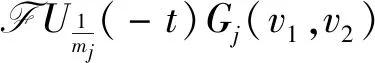
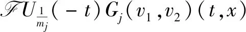
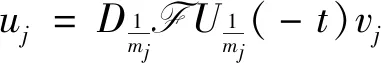
LetUα(t)=F-1E(t)αFwithα≠0,where the Fourier transform offis

and the inverse Fourier transform ofgis

The evolution operatorUα(t)and inverse evolution operatorUα(-t)fort≠0 are written as

and

respectively.These formulas are essential tools for studying the asymptotic behavior of solutions to the Cauchy problem (1) (see reference [10]).

which is represented as

fort≠0.Let[E,F]=EF-FE.We have the commutator relations

fors>0 (see reference [10]).

3 Proof of Theorem 1

We define the function spaceXTas follows

We start with the following lemma.

Lemma1Let 0

ProofBy the Cauchy-Schwarz inequality,we have

‖f‖L1(2)=‖f‖L1(|x|≤1)+‖f‖L1(|x|≥1)

So Little Three-eyes went to Little Two-eyes and said, I will go with you and see if you take good care of the goat, and if you drive him properly to get grass

=‖|x|-s1|x|s1f‖L1(|x|≤1)+‖|x|-s2|x|s2f‖L1(|x|≥1)

≤‖|x|-s1‖L2(|x|≤1)‖|x|s1f‖L2(|x|≤1)+‖|x|-s2‖L2(|x|≥1)‖|x|s2f‖L2(|x|≥1)

for 0

We next recall the well-known results (see reference [2]).

Lemma2Let 0≤s≤2,ρ≥2,then we have

forj=1,2,and

We set

forj=1,2.Therefore,from the Cauchy problem (1) we have

(11)

(12)

Lemma3We have

We next consider the estimate‖R2j‖L∞(2).By the definition ofR2jand Lemma 1,we get

where 0

By Lemma 3,we have the result from the inequality (12)

By the Lemma 2 and the existence of local solutions of the Cauchy problem (1),we have

≤Cε

whereT>1.Then we obtain

(13)

fort≥1,where 0

ProofWe have the identity

where 0

By Lemmas 2 and 4,we have the following lemma.

Lemma5We have

for anyt∈[1,T],where 0

ProofLet us consider the integral equation of the system (1),which is written as

(14)

forj=1,2.

By Lemma 4,we obtain

wheres=αorβ.This completes the proof of the lemma.

Lemma6There exists a smallδ>0such that

ProofLet

By the inequality (13) and Lemma 5,we get

Then we have

(15)

(16)

Since

by the inequality (16),we obtain

Thus we obtain

(17)

and by the inequality (17),we have

and

Thus we have

By Lemma 6,we have global existence of solutions to the Cauchy problem (1).We are now in the position of proving the time decay estimates of solutions to the Cauchy problem (1).From the equation (11),we have

(18)

(19)

By Lemma 3,Lemma 6,the equation (18) and the inequality (19),we obtain

(20)

By the Young inequality,we obtain

Thus we have

Integrating in time,we have

|u|≤C(logt)-1

(21)

fort≥2.

By Lemma 4,the inequality (21) and Lemma 6,we have

≤Ct-1(logt)-1