
Existence analysis of solutions of a class of cross diffusion equations on the mechanism of drug resistance of melanoma*
2023-06-01 07:20FENGZhaoyongLIUChengxia
中山大学学报(自然科学版)(中英文) 2023年3期
,,FENGZhaoyong,LIUChengxia
1. School of Applied Mathematics, Guangdong University of Technology, Guangzhou 510520, China
2. School of Mathematics, Sun Yat-sen University, Guangzhou 510275, China
3. Stomatological Hospital, Southern Medical University, Guangzhou 510280, China
Abstract: A mathematical model of checkpoint inhibitor targeted therapy for human melanoma is inves‐tigated.The model consists of twelve coupled reaction-diffusion equations, which includes free bound‐ary conditions and discontinuous terms.By transforming the free boundary problem into the fixed boundary problem, using the Lp theory of the parabolic equation and the Schauder fixed point theorem,and combining with the method of function approximation, the existence of the global weak solution of the mathematical model is obtained.
Key words: melanoma; reaction-diffusion equations; weak solution; existence
Human melanoma originates from melanocytes, and it is a malignant tumor of the skin.B-rafgene is one of the most common mutations in metastatic melanoma.Combining with the influence of drug resistance, Ascierto et al.obtained data from clinical trials, which showed thatBRAF-targeted therapy byBRAF-inhibitor would first s how obvious positive reaction, but usually relapses and becomes negative after half a year (Ascierto et al.,2012;Menzies et al.,2013;Sanchez-Laorden et al.,2014).Considering the factors of cell cycle parameters and age struc‐ture, Gaffney (2004) proposed a PDE model of the circulatory dynamics system, which mainly analyzed the ef‐fect of chemotherapy when drugs were used alternately.Steinberg et al.(2017) adjusted the chemotherapy regi‐men and medication strategy, and proposed different combination schemes forBRAFi, anti-CCL2 and checkpoint inhibitors.The purpose is to explore how to reduce drug resistance by combining drugs.Friedman et al.(2020)established a mathematical model corresponding to the experimental setup based on the existing experimental data (Steinberg et al.,2017).
The model comprises four cell equations, four chemokine equations and four drug equations(Friedman et al.,2020).Their concentrations are respectively denoted byC=C(r,t),M=M(r,t), etc., whereris a radial space variable satisfies 0 ≤r≤R(t), and the tumor radiusR(t) satisfies a differential equation.Besides,t≥0 is a time variable.We assume that the density of apoptotic or necrotic cell debris is constant.Then we consider the follow‐ing free boundary problem:
whereCis the density of cancer cells,Mis the density of macrophages (MDSCs),Dis the density of dendritic cells (DC),T8is the density of cells (CD8+T),Pis the density of catalytic factors (CCL2),I1is the density of inter‐leukin-10,I2is the density of interleukin-12,Nis the density of nitric oxide (NO),Bis the density of anti-BRAF,A1is the density of anti-PD-1,A2is the density of anti-PD-2,A4is the density of anti-PD-4.Moreover the coeffi‐cients are non-negative constants, ℜD(t) and ℜP(t)are nonnegative decreasing bounded continuous functions(p.14 (Friedman et al.,2020)).We can assume that some other variables express the following four dynamic equations in this paper, i.e.,P1=ρ1T8,P2=ρ2T8,P3=ρ3(T8+M+εCC),B7=ρ7D, so thatP1,P2are propor‐tional toT8(p.4 (Cui,2005)),P3is expressed on activatedT8,MandC,B7is proportional toD.Therefore, we do not need to deal with these four variables directly in this paper.
According to Friedman et al.(2020), the boundary conditions of the model is no flow boundary as follows :
We assumed that inactiveT8cells have a constant densityT̂8at the free boundary of the tumor, they are activated byI2when they enter the tumor environment (Friedman et al.,2020).Then we have the following boundary flux conditions
LetU0indicate the initial condition of these variables, a.e.,
it is clear thatU0is a nonnegative array (p.11 (Friedman et al.,2020)).In addition, we denoteR0=R(0).
In this paper,His an approximated Heaviside function (Friedman et al.,2020)
Obviously, it can be checked easily thatH(M−M0) is Lipschitzcontinuous.We assume a logistic growth forCwith carrying capacityCM, such that 0 ≤C≤CMand Δrrepresents the radial Laplacian, i.e.,
We assume the total density of cells in the tumor remains constant in space and time (Friedman et al.,2020):
and we assume that all cells have approximately the same diffusion coefficients.Adding Eqs.(1)-(4) and using Eq.(18), we get
where
andu(0,t) = 0.According to Friedman et al.(2020), there are some discontinuous items in this model, which in‐dicate the source of the drug:
whereγB,γA1,γA2andγA4are positive constants, indicating the level of drug efficacy.Obviously ΦB, ΦA1, ΦA2and ΦA4are bounded.It is not easy to deal with these discontinuous terms directly.Therefore, this paper draws les‐sons from the treatment method of parabolic equations with discontinuous terms in references (Cui,2005;Wei,2006;Wei et al.,2010;Xu et al.,2014), and intends to make a rigorous mathematical analysis of the model.
According to the biological principles, we have the following assumption:(A)U0≔(C0,M0,D0,T80,P0,I10,I20,N0,B0,A10,A20,A40) ∈Dp(0,1), the definition ofDp(0,1) is given in the fol‐lowing preliminary lemma.Besides,U0≥0.
Under the assumption (A), we obtain our main result as follows:
Theorem 1 The problem (1)-(17) has global weak solutions.
The structure of this paper is following.In section 1, we will present some preliminary lemmas which will be used in the following proofs.In section 2, we will transform the free boundary problem (1)-(17) into an equivalent problem on a fixed domain, which have some discontinuous terms in the model.We will focus on proving the existence of a fixed boundary problem after smoothing.And we prove that the initial-boundary value problem has global weak solutions in the last section.
1 Preliminary lemmas
In this section, we will present some preliminary lemmas.We first introduce some notations:
(i)QT={(r,t) : 0 ≤r≤1, 0 ≤t≤T},T> 0.QˉTis the closure ofQT.

2 Existence of approximate solutions
In order to solve the free boundary problem (1)-(17), we firstly transform it into an initial-boundary value problem in the fixed domain (z,τ), 0 ≤z≤1, 0 ≤τ≤T.Therefore, we introduce a transformation of variables(C,M,D,T8,P,I1,I2,N,B,A1,A2,A4) →(C′,M′,D′,T8′,P′,I1′,I2′,N′,B′,A1′,A2′,A4′),
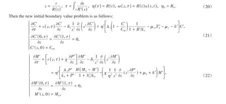
We summarize the above result in the following lemma.
Lemma 2 Under the variable substitution of (20), the problem (21)-(36) is equivalent to the problem(1)-(17).
Considering the discontinuous terms in problem (29)-(32), we can use smooth functions to approximate the discontinuous terms.In this case, these smooth functions (ΦB)ε, (ΦA1)ε, (ΦA2)εand (ΦA4)εare the approximations of discontinuous terms ΦB, ΦA1, ΦA2and ΦA4, respectively inC(0,T).The selection functions are as follows
Clearly, (ΦB)ε, (ΦA1)ε, (ΦA2)ε, (ΦA4)εare Lipschitz continuous inQˉT.Therefore, variables (C′,M′,D′,T′8,P′,I′1,I′2,N′,B′,A′1,A′2,A′4) can be approximated byU=(C′ε,M′ε,D′ε, (T′8)ε,P′ε,(I′1)ε, (I′2)ε,N′ε,B′ε,(A′1)ε,(A′2)ε,(A′4)ε).
Lemma 3 For anyT> 0, the problem (21)-(34) has solutions (Uε(z,τ),η(τ)) under the approximation.For convenience, we denoteU=(C′ε,M′ε,D′ε, (T′8)ε,P′ε, (I′1)ε, (I′2)ε,N′ε,B′ε, (A′1)ε, (A′2)ε, (A′4)ε), whereUε(z,τ) ∈W2,1p(QT),η(τ) ∈C[0,T].
Proof For a givenT> 0 and a positive constantGto be specified later,Gis independent of the values ofzandτ.We introduce a metric space (XT,d) as follows: the setXTconsists of a vector function (U(z,τ),η(τ)), (0 ≤z≤1, 0 ≤τ≤T) satisfying the following condition:


HereCp(T) is a positive constant depending onT,p,λ1,λ2,λ3,D0,T80andC0.
In the following, for (C,M,D,T8,P,I1,I2,N,B,A1,A2,A4) ∈XT, we define a mappingF: (U(z,τ),η(τ)) ↦(U͂(z,τ),ῆ(τ)).Given (U(z,τ),η(τ)) ∈XT, we define (U͂(z,τ),ῆ(τ)) to be the solutions of the following prob‐lems:
In the sequel, we will prove that (39)-(52) have global solutions by using Schauder fixed point theorem.
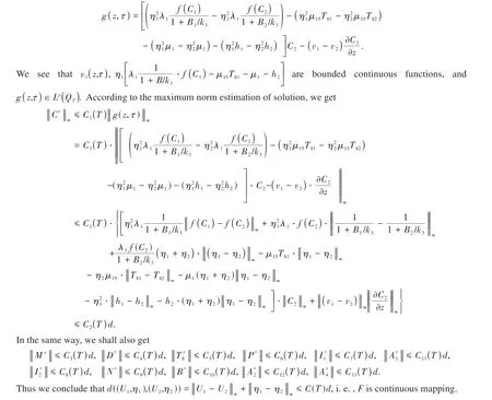
Step1 First, we need to prove thatFis a mapping fromXTtoXT.If (U,η) ∈XT, it is clear that (51)-(52)has a unique solutionῆ∈C[0,T], and
andU͂ε,ῆ satisfy (39)-(52).Obviously,Eis a closed convex subset ofXT.

In summary, we can prove that the mappingFhas a fixed point onEby using the Schauder fixed point theo‐rem, and the global solution can be obtained from the arbitrariness ofT.So Lemma 3 is proved.
3 The existence of solutions to original problem
In this section, we will use the function approximation method to prove the original problem has weak solu‐tions.
Lemma 4 For eachT> 0, (1)-(17) has weak solutions (U,η) =(Uε,ηε) onXT.
Proof Applying Lemma 3, we obtain that (21)-(32) exist weak solutionsUεunder the approximation,which satisfyUε∈W2,1p(QT).Therefore, by Sobolev's compact embedding theorem, we see that

For each (z,τ) ∈QT, εk→0, ask→∞, if we denoteUk=Uεk, then

Furthermore, the drugA1is depleted in the process of blockingPD−1 (p.9 ( Friedman et al.,2020)), so once the drug injection is stopped, there isA1= 0 instantly.By (61) it follows that
Hence
In the same way, we can also obtain
By the above analysis, Lemma 4 is proved.
In summary, by Lemma 2-4 and the arbitrariness of timeT, we see that Theorem 1 immediately follows.
