Improved Staggered Algorithm for Phase-Field Brittle Fracture with the Local Arc-Length Method

Zhijian Wu,Li Guoand Jun Hong

Jiangsu Key Laboratory of Engineering Mechanics,Department of Engineering Mechanics,School of Civil Engineering,Southeast University,Nanjing,214135,China

ABSTRACT The local arc-length method is employed to control the incremental loading procedure for phase-field brittle fracture modeling.An improved staggered algorithm with energy and damage iterative tolerance convergence criteria is developed based on the residuals of displacement and phase-field.The improved staggered solution scheme is implemented in the commercial software ABAQUS with user-defined element subroutines.The layered system of finite elements is utilized to solve the coupled elastic displacement and phase-field fracture problem.A one-element benchmark test compared with the analytical solution was conducted to validate the feasibility and accuracy of the developed method.Our study shows that the result calculated with the developed method does not depend on the selected size of loading increments.The results of several numerical experiments show that the improved staggered algorithm is efficient for solving the more complex brittle fracture problems.

KEYWORDS Phase-field model;brittle fracture;crack propagation;ABAQUS subroutine;staggered algorithm

Highlights

An improved staggered algorithm that uses the local arc-length method is formulated and proposed.

The energy and damage tolerance convergence criterion are employed in the numerical implementation.

The proposed algorithm results are not dependent on the selected sizes of the loading increments.

1 Introduction

Brittle fracture is one of the most feared failure modes in solids and structures.The numerical simulation method of brittle fracture is significant in engineering applications.Numerical simulation models for crack growth problems are generally divided into discrete crack models and diffuse crack models.The discrete crack model is a geometric description method based on mesh extension,which extends on mesh and mesh boundaries,including the element deletion method[1,2]and the interface element method[3,4].The element deletion method is a relatively simple fracture modeling method.It only needs to take the stress of the element zero or remove the mass of the fracture element from the overall mass matrix when a particular physical quantity associated with the element reaches the fracture criterion.The element deletion method cannot resolve the crack bifurcation problem [2,5].The interface element method inserts interface elements at the interfaces between elements,and there is cohesion between nodes of interface elements.When the fracture criterion is reached,the interface element fails and is broken.The interface element method only allows cracks to propagate at the element boundary, with apparent mesh dependence [5] and numerical instability.The diffuse crack model, including the extended finite element method (XFEM) [6–8] and the phase-field fracture method[9,10]is a nongeometric description method that can be separated from the mesh and expanded within the mesh.The XFEM allows cracks to expand inside the element by adding degrees of freedom to the nodes.The XFEM can be used to solve some simple fracture bifurcation problems in combination with existing bifurcation criteria [11–13].However, it is still challenging to simulate arbitrary crack propagation in three-dimensional problems.The difference between the XFEM and phase-field fracture method lies in the crack surface tracking technology deployed by the complex crack systems simulation method.XFEM is a discontinuous interface method requiring special crack tracking techniques to catch crack surfaces, such as level sets [14] and fast marching [15].These methods are particularly complicated when addressing three-dimensional and multicrack problems.

The research field of phase-field fracture models can be divided into the field of physics and the field of mechanics.The physical basis of the phase-field fracture models are based on the Ginzburg-Laudau theory,as shown by the model proposed by Hakim et al.[16].The phase-field fracture model in mechanics is based on the variational fracture approach developed by Francfort et al.[17] and is an extension of the traditional Griffith’s brittle fracture.Bourdin et al.[18,19] realized the rateindependent variational principle of diffuse fracture numerically for the first time.The diffuse phasefield boundary is employed to describe sharp crack boundaries.The phase-field fracture model is described by introducing order parameters and using continuous functions and controls the evolution of order parameters through the phase-field governing equations.Therefore,the phase-field fracture model obtains the path and location of the crack through automatic evolution of the phase-field variables without tracking the geometry of the crack[20,21].Crack propagation is controlled by the principle of free energy minimization for the phase-field fracture model[22,23].

In terms of algorithm implementation, the phase-field crack model can be solved with either a monolithic algorithm [24,25] or a staggered algorithm [26,27].In a monolithic algorithm, the displacement field and phase-field are solved simultaneously [28,29].However, the two fields are calculated separately in the staggered algorithm.Due to the strong nonlinearity of the partial differential equations, however, the monolithic algorithm requires a large number of iteration steps.The elastic strain energy decomposition method based on strain spectrum decomposition enhances the nonlinearity of the equations,and a monolithic algorithm often results in divergent consequences[30–33].A staggered method was developed by Miehe et al.[34]with a single staggered iterative process.It is widely used due to its simple implementation and strong robustness[35,36].To alleviate the problem of the common single iteration staggered algorithm, Karlo et al.[37] presented a comprehensive discussion on the use of a stopping criterion within the broadly used staggered algorithm that imposes the Newton-Rapson incremental loading procedure.

Nevertheless, the Newton-Rapson incremental loading procedure has difficulty capturing the complete failure process and the entire load-displacement curve because of the rapid failure of the structure due to the large loading step.To obtain accurate results, however, a small loading increment is necessary for the staggered algorithm.Several loading algorithms can track the whole load-displacement curve well,such as the global arc-length method[38,39],local arc-length method[40],energy dissipation control method[29,41],fracture surface control method[10,42],and J integral control method[43].Wu[44]proposed an iterative alternate minimization algorithm enhanced with path-following strategies which is based on the fracture surface control and the indirect displacement control.For the construction of complex engineering symmetric curves and surfaces in 2D and 3D phase-field modeling, an efficient method can be considered.Muhammad et al.[45] proposed a novel approach of hybrid trigonometric Bézier curve and applied it to engineering and computer aided design/computer aided manufacturing [46].The efficient modeling techniques and processes are helpful for computational models.

In this work,the phase-field method based on the rate-independent variational principle of diffuse fracture is considered.The formulations of the staggered algorithm with the local arc-length method are derived and proposed to avoid the sensitivity to the local failure of the structure and the softening of materials.The energy and damage iterative tolerance convergence criterion based on the residual norm of the displacement and phase-field is proposed to save computing resources.

The method of separating the node and degree of freedom of the element is employed to implement the improved staggered algorithm in the ABAQUS package, and they were alternating between the phase-field degree of freedom and displacement degree of freedom.An energy and damage iterative tolerance convergence criterion is embedded in each incremental loading of the local arc-length method.A one element benchmark test compared with the analytical solution was conducted to validate the feasibility and accuracy of the developed method.Several numerical experiments are conducted to simulate crack initiation,intersection,coalescence,branching,and propagation.

The paper is organized as follows.The representation of the phase-field approximation of diffuse crack topology is outlined in Section 2.1.The phase-field formulation for brittle fracture and classical staggered algorithm with Newton-Raphson method is derived in detail in Sections 2.2 and 2.3.The improved staggered solution for phase-filed with the local arc-length method and the implementation in ABAQUS/UEL, which includes the whole solution process, are discussed in detail in Section 3.Several static and dynamic benchmark tests and numerical examples are simulated and compared with other existing results in Section 4.Finally,conclusions are presented in Section 5.

2 Brief Review of the Phase-Field Model for Brittle Fracture

2.1 Representation of the Phase-Field Approximation of Diffuse Crack Topology

First,a simple model is considered to introduce the variational principle of diffuse crack topology.A cracked 1D bar with cross sectionΓand lengthL∈[–∞,+∞]is depicted in Fig.1a.Assuming that there is a fully opened crack at x=0,Γcan represent the crack surface that is completely broken.In this work, the auxiliary variablesφ(x) = [0,1] were employed to describe this sharp topology.Whenφ= 0, broken materials are present, whereasφ= 1, unbroken materials are present.The following exponential function[9]is used to approximate the nonsmooth(diffuse)phase-field:

wherel0is a regularization parameter describing the actual width of a diffuse crack.The axial crack in Fig.1b can be transferred into Fig.1c employing the phase-field approximation of the diffuse crack.Regularization is determined byl0.According to Fig.1b, considering the Dirichlet-type boundary conditionsφ(0)=1 andφ(±∞)=0.The solution of the homogenous PDE can be written as:

The one-dimensional description of the diffuse crack topology can be directly extended to the multidimensional case.According to the derivation process,the surface density functionγ(φ,▽φ)of cracks in unit volume can be expressed as:

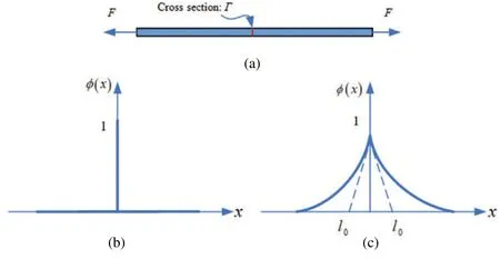
Figure 1:Sharp and diffuse crack topology(a)Cracked 1D bar(b)Sharp crack(c)Diffuse crack

Assume that we are given a sharp crack surface topology in Ω,as shown in Fig.2a.The regularized crack phase-field in the domain Ω can be obtained according to the minimization principle below(as shown in Fig.2b).

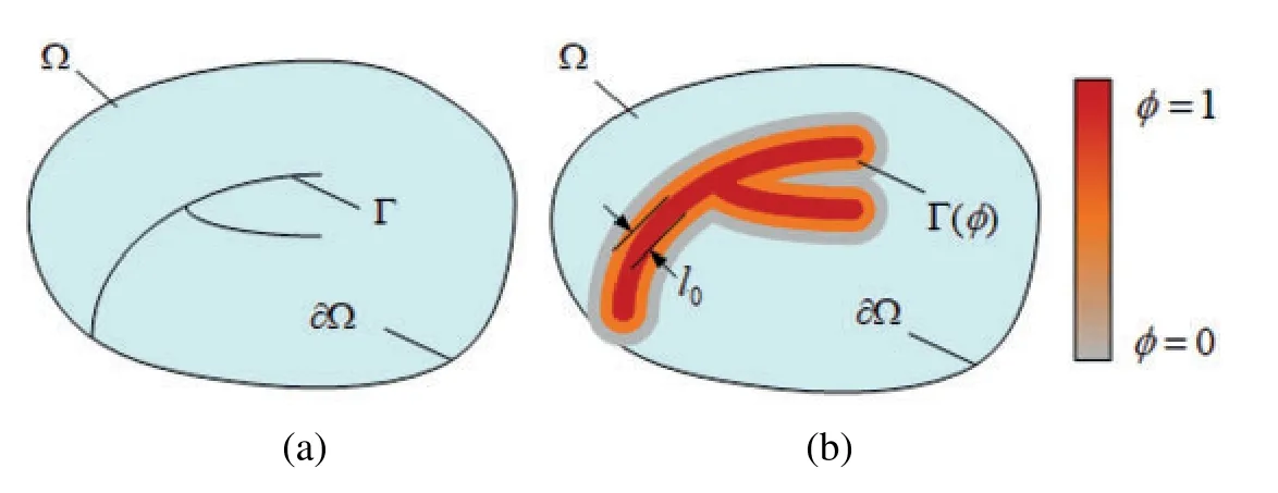
Figure 2:(a)Discontinuous discrete crack surface(b)Diffuse crack surface expressed by the phase-field variable

Francfort et al.[17]proposed a variational fracture model based on Griffith’s energy theory.The total potential energyof elastic solids consists of two parts:elastic energyEband crack surface energyEs:

whereψe(ε(u))is the elastic strain energy density function,ε(u)is the strain tensor,u∈Rd(d∈{1,2,3})andGcis the critical energy release rate.The variational model considers that at time t∈[0,T], the initiation,propagation,and branching of cracks at any location should minimize the total potential energy and meet some irreversible condition;namely,once a crack has formed,it cannot be restored.The regularized surface energy can be written as:

Assuming that linear elasticity exists in the unbroken solid, the elastic energy density can be calculated as:

where C0is the material linear elastic stiffness matrix.Elastic energy degradation due to damage follows the function:

the elastic energy density can be rewritten as:

According to the above fracture variation criterion, the surface energy of cracks results from elastic strain energy,that is,elastic strain energy drives the evolution of the phase-field variables.If the elastic strain energy is not decomposed,it will cause false branching of the crack.Given this problem,this work,based on the method proposed by Miehe et al.[23],observes the tension and compression decomposition of the elastic strain energy occurring so that the tension component of the elastic strain energy drives the evolution of the phase-field.The spectral decomposition of the strain tensor and elastic energy density is carried out via:

whereλandμare Lame constants.To correctly calculate the reduction effect of the phase-field variables on the stiffness of the material, assuming that the phase-field variables only affect the stretched part of the elastic strain energy density,the elastic strain energy density can be expressed as:

where the k ∈[0,1)is a model parameter used to avoid numerical singularity whenφ=1.

Considering the crack surface energy expression in Eq.(3) and the elastic strain energy density expression in Eq.(6),and considering the kinetic energy Ek as:

We can substitute part of the energy into the variational principle expression,to obtain:

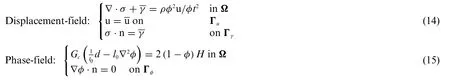
whereanddenote the body and face forces,respectively,and n is the unit outward normal vector.The minimization of the internal potential energy relative to the phase-field is now considered.In order to introduce the irreversible condition of damage,the historical field variableHneed to be introduced:

Htis the previously calculated energy obtained in history according to the displacement field ut at the time increment t.

By defining the change in external and internal potential energy and introducing the principle of virtual displacement,the governing equations of the model are obtained:

In order to obtain the numerical solution of the partial differential Eqs.(13)and(14),the finite element method is used to deal with the weak form more conveniently.

2.2 Discretization

In 2D space,the displacement field and the phase-field can be discretized as:

where the shape function matrix is expressed as:

then it is possible to express the gradients:

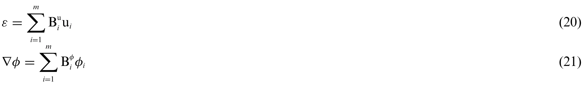
The strain-displacement matrices are expressed as:

According to the above expression, the residual of the discrete equation corresponding to the equilibrium condition for the displacement field and the crack phase-field can be expressed as:

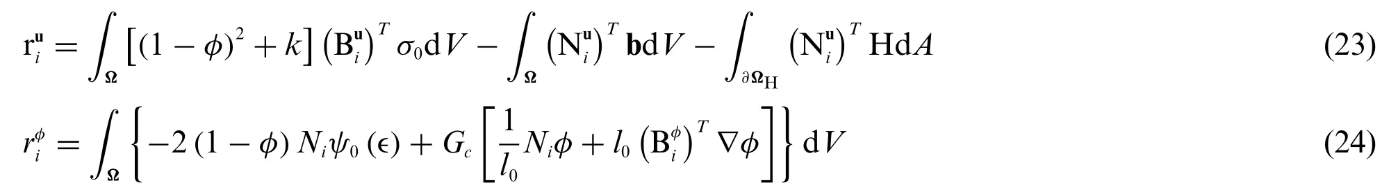
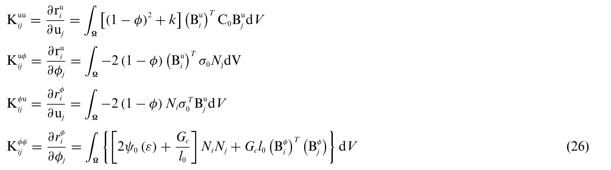
To obtain the solutions ofru= 0 andrφ= 0, and considering that their residuals are nonlinear,the incremental iteration scheme of the Newton-Raphson method is adopted.

where the static tangent matrices are calculated as:

2.3 Classical Staggered Algorithm with Newton-Raphson Method

In the case of unstable crack growth,the monolithic model is prone to convergence problems.The stress fields are rearranged due to the newly degenerated stiffness matrix when the crack propagates.Therefore, the solver cannot obtain a stable equilibrium solution.To obtain a stable model, the displacement field u and phase-fieldφof the coupled system can be solved as sequential coupled staggered fields.The phase-field and displacement fields in the staggered scheme are coupled variable fields.Furthermore,the calculation of the current history field is the main idea for the algorithmic split of the coupled equations,and it enforces the irreversibility of the evolution of the crack phase-filed.Consequently,the history field satisfies the Kuhn-Tucker conditions,

for both loading and unloading cases.Thus,no penalty term is needed in contrast to the monolithic approach.The residual corresponding to the evolution of the crack phase field is then as follows:

Similarly,the residual corresponding to the displacement field is then as:

The following system of the equation can be solved iteratively by employing the Newton-Raphson method,in which the tangent stiffness matrices are calculated as:

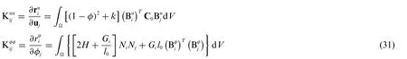
The new formula generates the above decoupling equations for sequential phase and displacement fields.Then,a staggered scheme of phase-field model is proposed.The displacement,phase and history fields ut,φtandHtare known at the previous time increment t.Then,the prescribed load vectors b are updated at the current time increment t +Δt.The current phase-fieldφt+Δt and the current displacement fieldut+Δt are now computed using the corresponding linear algebraic Euler equations.

3 Improved Staggered Solution Scheme with the Local Arc-Length Method

In this section,the improved staggered algorithm with the local arc-length method formulations and the corresponding numerical implementation are established.The local arc-length method [40]is applied to combine the staggered solution scheme with the energy and damage iterative tolerance convergence criterion.

3.1 Formulations of the Local Arc-Length Method

The arc-length method adjusts the external force loadfor displacement loadχto the convergence trend by constructing a scaling parameterλduring the loading process.The size of the loading step can be expressed in simple linear form as follows:

whereSis the weight function.

After linearization by the Newton-Raphson method, the residual Eqs.(25) and (26) are transformed into:

where the expressions of tangent stiffness are as follows:

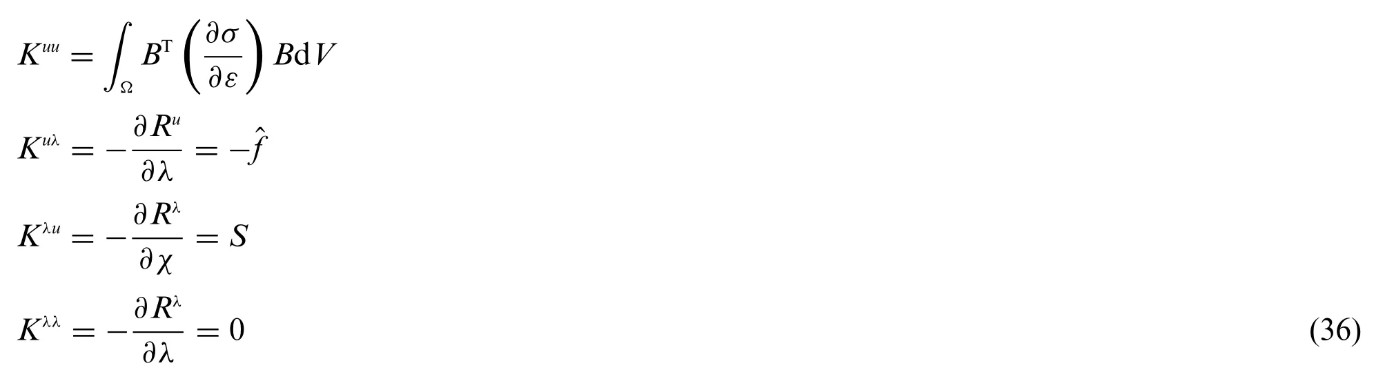
The unknown increment can be obtained by the following formula:

According to the Sherman–Morrison formula,Eq.(30)can transfer to:

whereχI andχII are obtained from the following equilibrium equations and correspond to the displacement of the node caused by residualsRuand the external forcef,respectively.

3.2 Staggered Algorithm with the Local Arc-Length Method and Its Numerical Implementation

Using the Newton-Raphson backward Euler scheme means that the numerical solution is unconditionally stable;that is,to achieve convergence means to obtain an equilibrium solution.Therefore,the solution is independent of the time increment.In the classic staggered scheme,the phase and the displacement fields are solved independently.This is unlike the monolithic case, where convergence is fulfilled for both coupled fields simultaneously, retaining unconditional stability.By solving for the phase and the displacement fields independently,the staggered scheme can track the equilibrium solution in a semi-implicit method, leading to a more robust numerical implementation.However,load increment sensitivity studies should be conducted.The residual staggered algorithm is improved to reduce the influence of the loading increment step on the solution process.The flowchart of the improved staggered solution scheme with the local arc-length method is shown in Fig.3.

Expression (37) is solved for the phase-field and the displacement field.The displacement field can be solved by the local arc-length loading method.The loading increment and iteration step should be distinguished in solving the displacement field.In some nonlinear analyses,the total load of each analysis step is decomposed into smaller incremental steps.The convergence results are obtained under a small incremental load to carry out the next step.The iteration step attempts to find a balanced solution in the loading increment step.At time increment t,andare built fromφt,andandare built fromut.When load increment step n is applied to load increment step n+1,Rut()can be calculated in the previous load increment step:

andrut(φnk)can be obtained in the form:

in then+1 load increment step,residuals are expressed as:

Then,following this process and repeating the iteration by assembling the residual stiffness matrixKtuu,Ktφφand combiningRutandRφt, ignores the effect of the load increment step directly.We obtain further verification from the numerical experiments section of this work.

By introducing the energy and damage convergence criterion, the improved staggered solution scheme is implemented to further improve the computational efficiency in solving phase-field brittle fracture problems.In the computation of the staggered solution,the solutions of the displacement field and phase-field both have their convergence criteria.

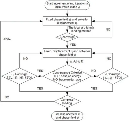
Figure 3:Process for the improved staggered algorithm with the arc-length method based on the energy and damage convergence criterion

At the beginning of the calculation,the damage value is fixed to solve the displacement subproblem.The damage value can be solved by the local arc-length method.When the displacement field converges,the displacement field is taken as a known quantity,and the damage subproblem is solved.There are two boundary conditions for solving the damage subproblem.One is that the phase-field is bounded, which isφ∈[0,1], and the range of the unknown quantity needs to be constrained in the process of solving.The other is that to ensure the irreversible condition of damage evolution ˙d≥0,the lower bound of the damage solution must be monotonically increasing.There are two kinds of convergence criteria adopted in this paper,one is based on the damage,and the other is based on energy:

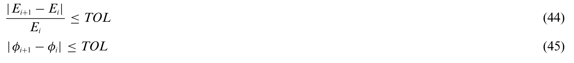
The process for the improved staggered algorithm based on the double convergence criterion is shown in Fig.3.The Expression (44) is the energy convergence criterion, while Expression (45)is the damage convergence criterion.The improved staggered algorithm considers both the energy convergence criterion and the damage convergence criterion.Once one of the convergence criteria reaches the corresponding tolerance, the program will continue to calculate the next iteration step.TOLis the tolerance of convergence,generally 10–5.For materials with strong brittleness,TOLshould be lower;otherwise,the peak point may be lost.In the actual solution process,when the structure is in the linear elastic state,there is only one staggered solution process for each loading step.However,when the structural response enters the nonlinear state, because of the strict convergence criterion of the staggered solution algorithm, multiple staggered solution iterations are often needed in one loading step.

The core of the traditional staggered solution scheme is to fix the phase-fieldφand solve for the displacementu, fix the displacementuand solve for the phase-fieldφ, and repeat the cycle until convergence.In addition to the conventional displacement degree of freedom, the degree of freedom of the finite element node needs to be added to the phase-field, and it is realized from the perspective of a multifield finite element.The alternating process of the phase-field degree of freedom and displacement degree of freedom can be realized in the following three ways:

1.Add the phase-field element and displacement element.The corresponding degrees of freedom are given in the staggered solution process.

2.Add the phase-field element.Two submodels with the same mesh division should be established,one of which is the displacement element and the other being the phase-field element.In the staggered solution scheme,submodels are called for solutions.

3.Separate the node and the degree of freedom of the element.Set the element type without the degree of freedom in the model file,and then give the element’s corresponding node the degree of freedom in the solution process.

Regarding program expansibility and simplicity,the third method is best.The phase-field brittle fracture model can be solved directly in the finite element framework.The commercial software ABAQUS is employed to solve the iteration process and realize the improved staggered algorithm for phase-field modeling.

The layered system of the finite element implemented in ABAQUS with UEL and UMAT is shown in Fig.3.The process for solving the phase-field model in each layer is described in detail in Fig.4.

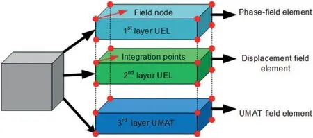
Figure 4:Schematic illustration of the 3-layered element structure in ABAQUS with its subroutine

Since the phase-field equation and the balanced equation are solved separately,the implicit solver ABAQUS/Standard or the explicit solver ABAQUS/Explicit can be flexibly selected according to the model when solving the displacement field.The former is implemented through the UMAT subroutine interface provided by ABAQUS,and the latter is implemented through VUMAT.

As depicted in Fig.4, the node and the integration points coincide in the phase-field model.The first layer of finite elements includes user elements implemented by the user subroutine UEL.The degree of freedomφi, is implemented instead of the ABAQUS rotation degree of freedom so that the phase-field residual norm and the residual displacement norm are entirely separated.The discretization matrices, stiffness matrix, and residual vector must be defined in the first layer.The second layer of finite element is for the displacement field.

The solution-dependent variables used to solve differential equations in two dimensions are listed in Table 1.The third layer is for the UMAT field element.Not only can it be used as a visualization tool,but it can also control the convergence of the iteration process.

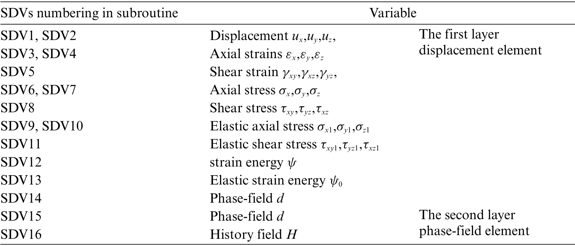
Table 1:List of solution dependent variables

4 Numerical Examples and Algorithm Validation

4.1 One Element Test

A finite element model with the UEL implementation should be developed to verify the feasibility of solving brittle fracture problems using the algorithm,as demonstrated through the most straightforward case in Fig.5.A 2D plate is extended on top in direction Y,whereas bottom nodes are constrained in both directions.As the dimensions of the square plate are 1×1 mm,the characteristic of the element is 1 mm.The material and fracture properties are chosen:Young’s modulus E=210 GPa,Poisson’sμ=0.3,critical fracture energy densityGc=2.7×10–3kN/mm,and length scale parameterl0=0.1 mm.

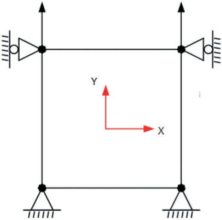
Figure 5:The plane strain element with boundary condition

This case is solved using 5 different displacementsΔu to reach u = 0.1 mm.The five-step displacements areΔu = 1 × 10–5,Δu = 5 × 10–5,Δu = 1 × 10–4,Δu = 5 × 10–4, andΔu = 1 ×10–3,corresponding to 10000 steps,2000 steps,1000 steps,200 steps,and 100 steps.Fig.6 shows the axial stress-strain response comparison of the numerical results of the traditional staggered algorithm and the improved staggered algorithm against the analytical solution.

According to Fig.6a,when the axial strain is close to 0.01,the axial stress reaches the maximum value.With the increase of strain,the error of stress increases in the rising stage and decreases in the falling stage.At the peak of the curve,the error of stress is at its maximum.The traditional staggered algorithm is strictly dependent on the size of the increment step.The smaller the increment is, the smaller the error between the numerical result and the analytical solution.That is when the crack starts to propagate and due to the quick stiffness and stress reduction in some elements,stability problems appear in the traditional staggered algorithm.According to Fig.6b,however,the numerical result of the improved staggered algorithm is independent of the increment step size.Regardless of the value of the increment step,the numerical solution can be in good agreement with the analytical solution.Similarly,according to Fig.7,the numerical solution of the governing phase-field evolution through the axial strain matches well with the analytical solution.Hence,the improved staggered algorithm is validated through the one element test.The results show that the improved staggered algorithm for phase-field brittle fracture with the local arc-length method efficiently solves brittle fracture problems.

Figure 6:Stress-strain curves obtained by(a)The traditional staggered algorithm and(b)The improved staggered algorithm in comparison with the analytical solution

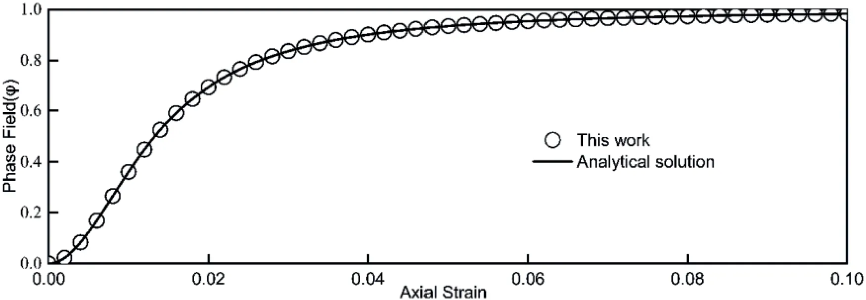
Figure 7:Comparison of the phase-field between the numerical and analytical results

4.2 Single Edge Notched Test

The single edge notched test is the most common test used to validate phase-field brittle fracture models.The geometry and the boundary conditions of the square specimen are depicted in Fig.8.The side length of the square is 1 mm,and the edge notched is horizontal from the middle of the left side to the center of the square.α=90°and theα=0°,corresponds to the pure tension case and pure shear case, respectively.The material and fracture properties are chosen:Young’s modulusE= 210 GPa,Poisson’sμ=0.3,critical fracture energy densityGc=2.7×10–3kN/mm,and length scale parameterl0=0.075 mm.

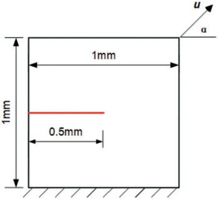
Figure 8:Geometry and boundary conditions of a single edge notched specimen

Fig.9 shows the fracture pattern for unidirectional tension(α=90°).Fig.10 shows the fracture pattern for pure shear(α=0°).The two fracture patterns in the improved staggered algorithm are in good agreement with the existing references[35].For unidirectional tension(α=90°),the crack begins in the center of the geometry and extends horizontally to the right side.For pure shear(α=0°),a crack path can be seen starting withβ=61°from the deformation direction.

Figure 9:Crack patterns for the single notch edge tension test at different displacements

Fig.11 shows the reaction force in tensile specimens, along with the results of Miehe et al.[9].The maximum reaction force value is consistent,and only a small deviation can be observed during crack propagation.In the rising stage, the error of the reaction force is small.The large error in the descending stage mainly comes from the selection of mesh density.

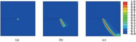
Figure 10:Crack patterns for the single notch edge shear test at different displacements

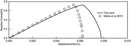
Figure 11:Reaction force in the single notched edge tension test

In addition to the quasi-static crack propagation of the 2D model, the 3D model of the single edge notch test is solved using the same parameter.The geometry and boundary conditions for the 3D single edge notched tensile modeling are depicted in Fig.12.The number of solution dependent state variables of two dimensions are different from the three dimensions due to the z-direction degree of freedom,which is defined as 26 SDVs.The crack starts at the end of the initial crack in the middle of the specimen and ends at the right boundary of the specimen,similar to the two-dimensional model.The crack patterns for the single notch edge tension test of the 3D model at different displacements are shown in Fig.13.The case shows that the improved staggered algorithm for phase-field brittle fracture with the local arc-length method is efficient for solving brittle fracture problems in pure tension and shear situations in the 2D model and the 3D model.

4.3 Notched Bimaterial Tensile Test

This case study is a tensile sample of two materials.The upper material is harder,while the lower material is 10 times softer and has an initial notch.The sample is tensioned parallel to the separation line.The geometry and boundary conditions are shown in Fig.14.The upper material properties are chosen:Young’s modulusE=210 GPa,Poisson’sμ=0.2,and critical fracture energy densityGc=1×10–2kN/mm.The lower material properties are chosen:Young’s modulusE=3.77 GPa,Poisson’sμ=0.2,and critical fracture energy densityGc=1×10–3kN/mm.

The purpose of this benchmark test is to show that our implementation can model the crack branching phenomenon.Fig.15 shows the crack patterns for the bimaterial tensile test at different displacements.After the crack begins,it normally propagates until it reaches the material transition zone.Then,because it takes less energy to branch over a short period of time than it does to continue into the upper hard material,the damage zone becomes larger,and the cracks separate along with the interface between the upper and lower material.

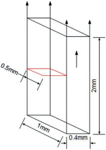
Figure 12:Geometry and boundary conditions for the 3D single edge notched tensile test

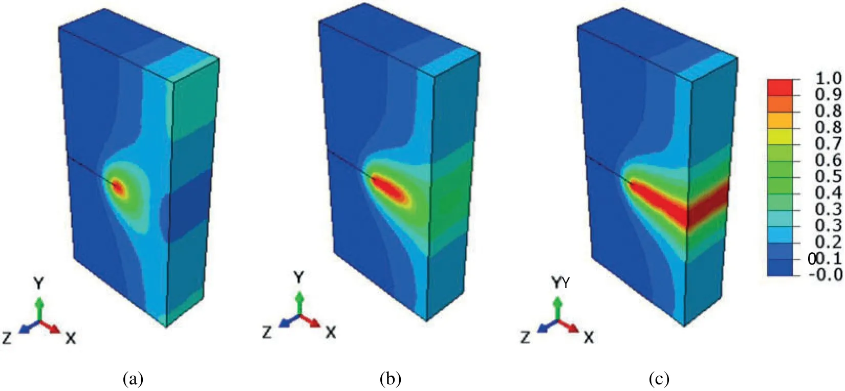
Figure 13:Crack patterns for the single notch edge tension test of the 3D model at different displacements

Since the purpose of this benchmark test is to show crack branching, the center of the finite element mesh is dense.As the local amplification region is showm in Fig.15,the cracks spreads along the direction of the crack,and the width of the crack decreases after separating along with the interface.As a result,cracks in harder materials are wider because the finite element size in this region is larger.This notched bimaterial tensile numerical experiment is conducted to simulate crack branching using the improved staggered algorithm for phase-field brittle fracture with the local arc-length method.

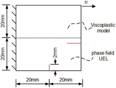
Figure 14:The geometry and boundary conditions for the bimaterial tensile test

Figure 15:Crack patterns for the bimaterial tensile test at different displacements

4.4 Symmetric and Asymmetric Double Notched Tensile Test

After the simple example,we will show a few more complex cases to demonstrate the utility of the new implementation.A symmetric and asymmetric double-notched specimen is used to investigate coalescence of cracks.Figs.16 and 18 depict the exact geometry.The following material properties are used:Young’s modulusE= 210 GPa, Poisson’sμ= 0.3, critical fracture energy densityGc= 2.7 ×10–3kN/mm,and length scale parameterl0=0.075 mm.

The crack patterns for symmetric and asymmetric doubled notched specimen tension tests at different displacements are shown in Figs.17 and 19.For asymmetric doubled notched specimen tension tests,the cracks expand simultaneously from the left and right sides.The upper crack extends downwards and the lower crack extends upwards and then meet in the center of the specimen.For symmetric doubled notched specimen tension tests, the cracks expand simultaneously from the left and right side,then meet in the middle and merge.The final fracture pattern is very consistent with the previous results.This symmetric and asymmetric double notched numerical experiment is conducted to simulate crack coalescence using the improved staggered algorithm for phase-field brittle fracture with the local arc-length method.

Figure 17:Crack patterns for symmetric doubled notched specimen tension test at different displacements

4.5 L-Shaped Specimen

The L-shaped specimen in[26]is taken as an example to simulate the evolution process of the crack path.The geometry and boundary conditions are shown in Fig.20.The following material properties are used:Young’s modulusE=28.8 GPa,Poisson’sμ=0.18,critical fracture energy densityGc=8.9×10–5kN/mm,and length scale parameterl0=1.1185 mm.A finite element mesh consisting of 52634 elements was used to refine the expected crack propagation region.The improved staggered algorithm is used for this specimen to demonstrate its ability in more complex geometry.

Fig.21 shows the phase-field and equivalent strain plots for the L-shaped specimen obtained from the phase-field fracture model at different displacements.The crack starts at the corner of the Lshaped plate and spreads slightly upward horizontally.The crack path is basically consistent with the path of equivalent strain plots.The results were compared with the experimental measurement results provided in [26].The calculated results of the crack growth process are convergent and consistent with the published experimental results.This L-shaped specimen numerical experiment is conducted to simulate crack propagation in more complex modeling using the improved staggered algorithm for phase-field brittle fracture with the local arc-length method.

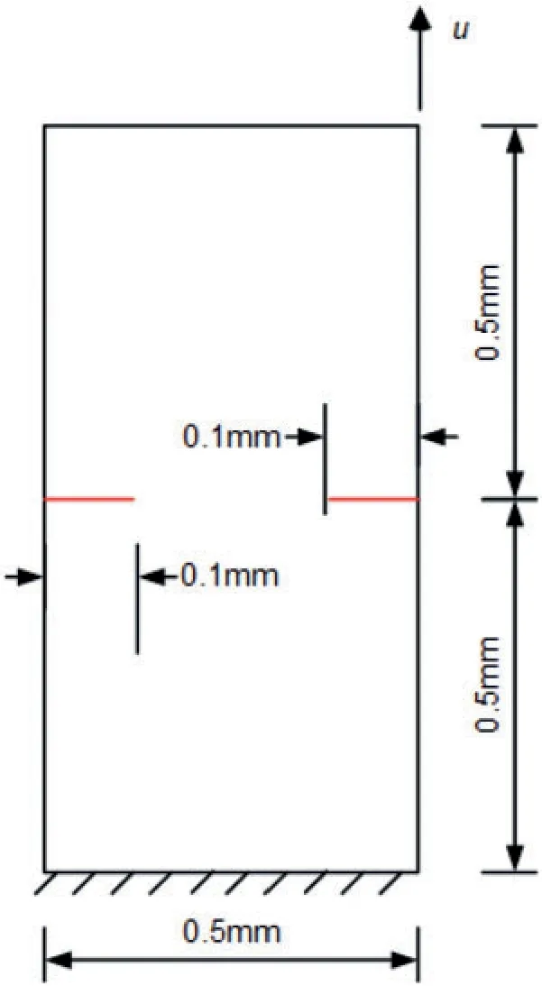
Figure 18:Geometry and boundary conditions of asymmetric doubled notched specimen

Figure 19:Crack patterns for the asymmetric doubled notched specimen tension test at different displacements

Figure 20:Geometry and boundary conditions of the L-shaped specimen

Figure 21:Phase-field and equivalent strain plots for the L-shaped specimen obtained from the phasefield fracture model at different displacements.(a)u=0.20 mm,(b)u=0.35 mm,(c)u=0.70 mm

4.6 Dynamic Crack Branching

In addition to the quasi-static crack propagation examples, dynamic crack propagation is also handled by means of the improved staggered algorithm.The geometry and boundary conditions of the dynamic crack branching are shown in Fig.22.An initial crack with a length of 50 mm was prefabricated in the middle of the plate, and the top and bottom sides of the plate were subjected to an impact load of 1 MPa.In order to reduce the errors of mesh size on the calculation results,the phase-field fracture modeling is composed of uniform quadrilateral elements with a size of 2.5×10–4.The material and fracture properties are chosen as:densityρ= 2450 kg/m3, Young’s modulusE= 32 GPa, Poisson’sμ= 0.18, critical fracture energy densityGc= 3× 10–3kN/mm,length scale parameterl0=0.01 mm,and Rayleigh wave velocityVR=2125 m/s.

The crack patterns for the dynamic crack branching are shown in Fig.23,and the velocity curve of the crack is shown in Fig.24.The crack will branch when it suffers the impact load.From the curve,the maximum velocity of the crack tip reaches approximately 0.5 VR,which is basically consistent with the results of the test.It is noted that the crack tip velocity branches immediately after reaching the peak for the second time,and the branching occurs from 30 μs and 36 μs.The velocity of the crack tip decreases immediately after crack branching and starts to increase again after 40 μs.Borden et al.[28]first applied the phase-field method to model the case.Song et al.adopted other fracture numerical methods for the same model.In this work, we compare the curve of the velocity of the crack tip propagation with the results of Borden’s test, which is solved in terms of the monolithic algorithm.The numerical results of the algorithm are in good agreement,and the velocity of the crack tip for the staggered method is slightly lower than that of the monolithic method.The phase-field fracture model does not require additional branch criteria or numerical iteration of discontinuous displacement fields when simulating dynamic crack branching and propagation.Compared with the XFEM,phase-field fracture modeling is more efficient.This dynamic branching numerical experiment is conducted to simulate dynamic crack propagation using the improved staggered algorithm,which applies not only to the quasi-static model but also to the dynamic model.

Figure 22:Geometry and boundary conditions for the dynamic crack problems

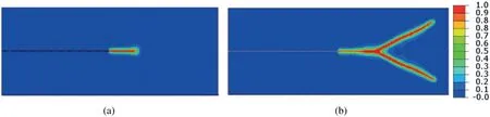
Figure 23:Crack patterns for the dynamic crack problems

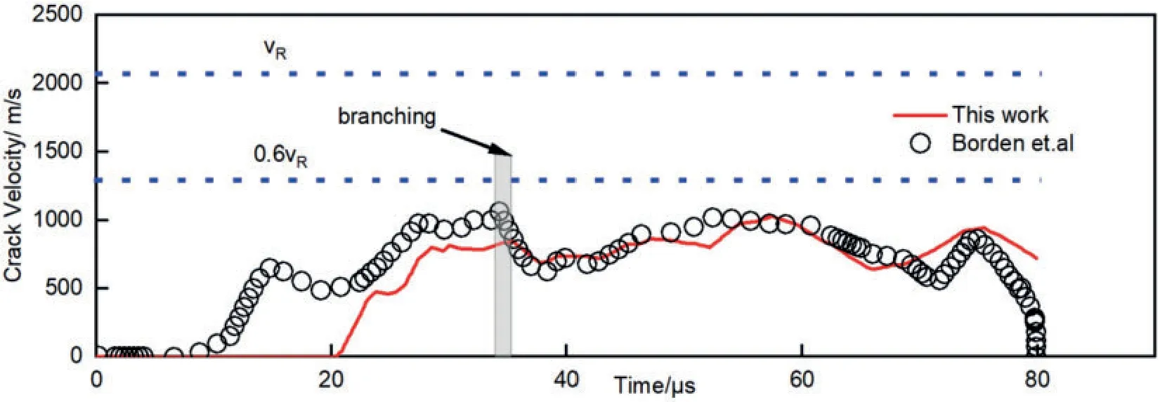
Figure 24:The crack tip velocity for the dynamic crack problems

5 Conclusions

In this study,an improved staggered scheme with the local arc-length method is proposed to study phase-field brittle fracture.The energy and damage iterative tolerance convergence criteria based on the residuals of displacement and phase-field is developed and implemented in ABAQUS.We adopt a one element benchmark numerical test and several numerical examples to verify the feasibility and accuracy of the phase-field model.From the presented work,the following conclusions can be drawn:

1.The local arc-length method applied to the staggered solution scheme of the phase-field brittle fracture can track the crack propagation process and load-displacement curve well.

2.The improved staggered scheme for brittle fracture is not sensitive to the size of the load increment.The accuracy and efficiency are greatly improved.

3.The results of one element benchmark test and several complex numerical examples are in good agreement with the other numerical solutions.

4.The improved staggered scheme for the brittle fracture model is an effective method to accurately simulate crack initiation,coalescence,intersection,and branching.

Funding Statement:Financial supports by the National Key R&D Program of China (No.2018YFD1100401), the National Natural Science Foundation of China (No.51578142), the Fundamental Research Funds for the Central Universities (No.LEM21A03), and Jiangsu Key Laboratory of Engineering Mechanics(Southeast University)are gratefully acknowledged.

Conflicts of Interest:The authors declare that they have no conflicts of interest to report regarding the present study.