Adaptive multiscale convolutional neural network model for chemical process fault diagnosis

Ruoshi Qin,Jinsong Zhao,2,*

1 State Key Laboratory of Chemical Engineering,Department of Chemical Engineering,Tsinghua University,Beijing 100084,China

2 Beijing Key Laboratory of Industrial Big Data System and Application,Tsinghua University,Beijing 100084,China

Keywords:Neural networks Multiscale Adaptive attention module Triplet loss optimization Fault diagnosis Chemical processes

ABSTRACT Intelligent fault recognition techniques are essential to ensure the long-term reliability of manufacturing.Due to the variations in material,equipment and environment,the process variables monitored by sensors contain diverse data characteristics at different time scales or in multiple operating modes.Despite much progress in statistical learning and deep learning for fault recognition,most models are constrained by abundant diagnostic expertise,inefficient multiscale feature extraction and unruly multimode condition.To overcome the above issues,a novel fault diagnosis model called adaptive multiscale convolutional neural network (AMCNN) is developed in this paper.A new multiscale convolutional learning structure is designed to automatically mine multiple-scale features from time-series data,embedding the adaptive attention module to adjust the selection of relevant fault pattern information.The triplet loss optimization is adopted to increase the discrimination capability of the model under the multimode condition.The benchmarks CSTR simulation and Tennessee Eastman process are utilized to verify and illustrate the feasibility and efficiency of the proposed method.Compared with other common models,AMCNN shows its outstanding fault diagnosis performance and great generalization ability.

1.Introduction

The chemical industry is full of high risks with the complexity of manufacturing facilities and the interaction of reactive substances.A fault in the chemical production process which is incorrectly identified and not handled in time will evolve into a major safety accident[1].Although a large number of measures and techniques have been applied in the actual industry to prevent system errors,such as distributed control system and safety instrumented system,abnormal situation management still relies on manual analysis and treatment by skilled operators[2].Therefore,effective fault diagnosis of chemical process is crucial to guarantee the safety and reliability of a system.Thanks to the implementation of advanced information technologies,a large amount of measurement data is available to assist in fault recognition.Plentiful datadriven models are developed constantly in academic studies in the past decade.

Data-driven fault diagnosis models are generally divided into statistical models and deep learning models.Statistical models evolve continually and succeed in processing the highdimensional,noisy and highly correlated data from chemical processes [3].Principal component analysis (PCA) [4] and its variants are one of the most popular dimensionality reduction techniques.Many researchers have improved this method and presented dynamic PCA [5],kernel PCA [6] and so on for application.Partial least squares (PLS) [7] is another powerful statistical tool which preserves the significant variability information of data.The updated versions including recursive PLS [8],and dynamic inner PLS[9]make progress in overcoming the nonlinear characteristics.Independent component analysis (ICA) [10],fisher discriminant analysis (FDA) [11],support vector machine (SVM) [12] and their developments are also widely used for monitoring.Apart from the above,some new statistical learning models are released lately.Zhanget al.[13]developed one kernel entropy component analysis classifier for each fault domain.Ziaei-Halimejaniet al.[14] combined recurrence quantification analysis and unsupervised learning clustering methods such as k-means and density-based spatial clustering to analyze the features influenced by faults.However,the statistical models heavily depend on the manually selected features which depend on considerable expertise and extensive mathematical knowledge.The reliance on manual experience imposes restrictions on generalizing these traditional models.

In recent years,a wide variety of deep learning models have been applied to diagnose chemical process faults.Alternate linear transformations and nonlinear activation functions enhance the nonlinear fitting performance of multi-layer artificial neural networks (ANN).Initially,some network structures derived from ANN were developed for fault recognition,such as hierarchical ANN [15] and ANN supplemented with expert knowledge [16].Since the rapid development of deep learning mechanisms,deep belief network (DBN) [17],variational recurrent autoencoder(VRAE) [18] and convolutional stacked autoencoder (SAE) [19]have been published separately.Zhanget al.[20] employed bidirectional recurrent neural network (BiRNN) for complex chemical processes in both positive and negative directions.Wuet al.[21]innovatively proposed a process topology convolutional network(PTCN) that merged data information and process knowledge.The PTCN model integrated the process topology into a graph reflecting the relationships among different variables.Biet al.[22] designed orthogonal self-attentive variational autoencoder(OSAVA) for process monitoring and performed fault detection and identification tasks simultaneously with interpretable results.Some novel generative adversarial network models were also applied to fault diagnosis tasks in current times [23].

Among those deep learning models,convolutional neural network (CNN)is a typical architecture based on feed-forward neural networks.The hierarchical units of CNN energize its abilities to perform translation-invariant classification of input so that CNN is demonstrated to be well adapted to fault diagnosis missions[24].CNN was first proposed for two-dimensional (2D) image recognition.To meet the input requirements of the traditional CNN structure,the one-dimensional (1D) time-series data is usually generated into images.Wu transformed historical data into sample matrices with corresponding labels and constructed a deep convolutional neural networks (DCNN) diagnostic model which extracted features in spatial and temporal domains simultaneously[25].The chemical process dataset contains multiple variables including temperature,pressure,liquid level and so on.Since different variables have different influenced factors,their fluctuation trends vary from each other under the regulation of the control system.Therefore,the features of a certain scale that reflect the variation of each variable cannot generalize the overall trend.More comprehensive features extracted at various scales can help fault diagnosis.However,the traditional 2DCNN is only capable of extracting features of a fixed scale,which prevents the multiscale feature learning ability and the adaptability of mode switching.Song created a multiscale CNN(MSCNN)model for state classification and converted the preprocessed data into matrix color diagrams as input [26].But it is considered that the primarily measured signals contain the inherent fluctuation characteristics which reveal the periodic information of faults more accurately.Zhanget al.[27] stated that 1DCNN model worked better on raw rotating machinery signals of changing loads compared to 2DCNN without handcrafted data pre-processing.It’s still rare to discover a practical chemical process fault diagnosis model so far that excellently captures the multiscale features from time-series data directly.

In addition to the problem of multiscale feature extraction,the variation of feed and environment brings about several operating modes in the chemical process.In order to capture more useful fault information from multiple data distributions,many creative multimode monitoring methods have been put forward.Wuet al.[28] delivered a self-adaptive deep learning method combining local adaptive standardization and variational auto-encoder bidirectional long short-term memory(LAS-VB)to achieve multimode feasibility.Zhenget al.[29] discovered a self-adaptive temporal-spatial self-training algorithm(SATSST)to solve the challenge of switching working conditions and inadequate data labels.Transfer learning is also utilized to realize the domain adaptation from the source mode to the target mode [30].Motivated by the successful application of attention mechanism in visual inspection,which is a recent topic of great interest to worldwide scholars,some improved approaches are adopted in the field of fault diagnosis.Miao presented adaptive densely connected convolutional auto-encoder (ADCAE) for gearbox signal feature learning [31].Yaoet al.[32] explored recursive attention mechanism (RAM)to strengthen the anti-noise acoustic-based classification performance.

Inspired by these observations,a fault diagnosis approach of chemical process based on Adaptive Multiscale Convolutional Neural Network(AMCNN)is proposed in this paper.The model designs a novel multiscale CNN to perform feature extraction and fault diagnosis on raw time-series data.A new adaptive attention module is embedded into the multiscale CNN structure to estimate the importance of extracted features so as to emphasize the useful ones.The entire deep network is optimized by a metric learning tool,the triplet loss optimization,which provides the model with strong power of discriminability and generalization in diverse operating conditions.

The remainder of this paper is organized as follows.In Section 2,the theoretical background and the overall fault diagnosis model are illustrated in detail.In Section 3,experimental studies are implemented to verify the effectiveness of AMCNN,and the presented model is compared with other published works in terms of fault classification performance.Conclusion and further discussion are indicated in Section 4.

2.Methodology

The proposed model includes three key parts: (1) multiscale convolutional neural networks for feature extraction from multivariate time-series data;(2) adaptive attention module for representative characteristics selection and (3) triplet loss mechanism for anomaly diagnosis optimization.The detailed principles of the above concepts are introduced in the following sections,followed by the summarization of the overall fault diagnosis model framework at the end of this section.

2.1.Multiscale convolution

As one of the most widely applied models in deep learning,CNN has been investigated in a variety of recognition tasks.Stacked convolutional layers and fully-connected layers endow the powerful model with automatic feature extraction and classification.CNN can deal with various types of signals and 1DCNN is able to address raw temporal data without any time-consuming preliminary conversion into matrix diagrams.The convolutional kernel is the key unit to extract data characteristics,and the size of the receptive field determines how much information can be obtained from the input signals.However,the general CNN models configured with the fixed kernel width are trapped in the same size of receptive,which means they can only take the single-scale features into account.As a result,it is undesirable to capture efficient features under variable operating conditions.

Motivated by the Inception modules of GoogLeNet network[33],multiple kernels of different sizes can be integrated to perform convolutional operations on one-dimensional signals,and multiscale features are extracted at the same time.Fig.1 reveals the differences between multiscale convolution models and the traditional convolutional networks,whereFstands for the feature information,Wthe kernel size andCthe number of channels.In contrast with the basic convolutional layer,a multiscale convolutional block consists of multiscale convolutions and a flat convolutional layer.The filter concatenation achieves the fusion of multiscale features.Larger convolutional kernels allow more efficient extraction of slowly varying components at wider time scales,while the smaller ones can detect the transient behaviors of the data under fluctuation.

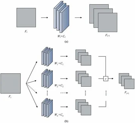
Fig.1.Architectures of different convolutional layers in CNN.(a) One convolution.(b) Multiscale convolutions.

The designed multiscale convolution architecture example is illustrated in Fig.2.A large-size convolutional kernel is introduced as the first layer of the network to seize the features of the lowfrequency band.The number of channels is dynamically adjusted with the requirements of the task data.The model contains two multiscale convolution modules to obtain more information from the raw measurements.Three main kinds of filters with the sizes of 1×1,1×3,and 1×5 are utilized to convolve with the characteristics accompanied by other large kernels as initial auxiliary.The multiple cascade channels facilitate the dimension reduction of the feature maps.The model robustness is further enhanced by embedding the maximum pooling operation with the subsampled vectors rescaled for further selection.In case of different classification tasks with multiple variables,the convolution kernel size and the amount of input and output channels need to be enlarged along with the increasing dimension of input data.

2.2.Adaptive attention module

The multi-attention module aims to select useful features automatically and suppress useless information extracted from the deep networks.Two revised attention mechanisms,adaptive channel attention and adaptive spatial attention,are activated successively and combined as a whole to enhance feature learning.

2.2.1.Adaptive channel attention

The application of the attention mechanism in channel mode is regarded as a solution to select the most sensitive feature channel for fault diagnosis [34].The adaptive channel attention algorithm shown in Fig.3 receives the feature maps obtained from the multiscale convolutions,and the one generated through theith kernel branch is defined as the feature mapFi.The global average pooling and max pooling are operated to acquire different channel descriptorswhich make the element corresponding to the feature in the certain channel squeezed through a spatial dimensionL×1.These descriptors contain different ranges of information and denote diverse characteristics.Then,a shared network composed of the multilayer perceptron (MLP) with a hidden layer is embedded to generate the selective weights on channels and integrate them into a channel attention mapMchannel∈RC×1×1.The module computes the element-wise summation in Eq.(1):

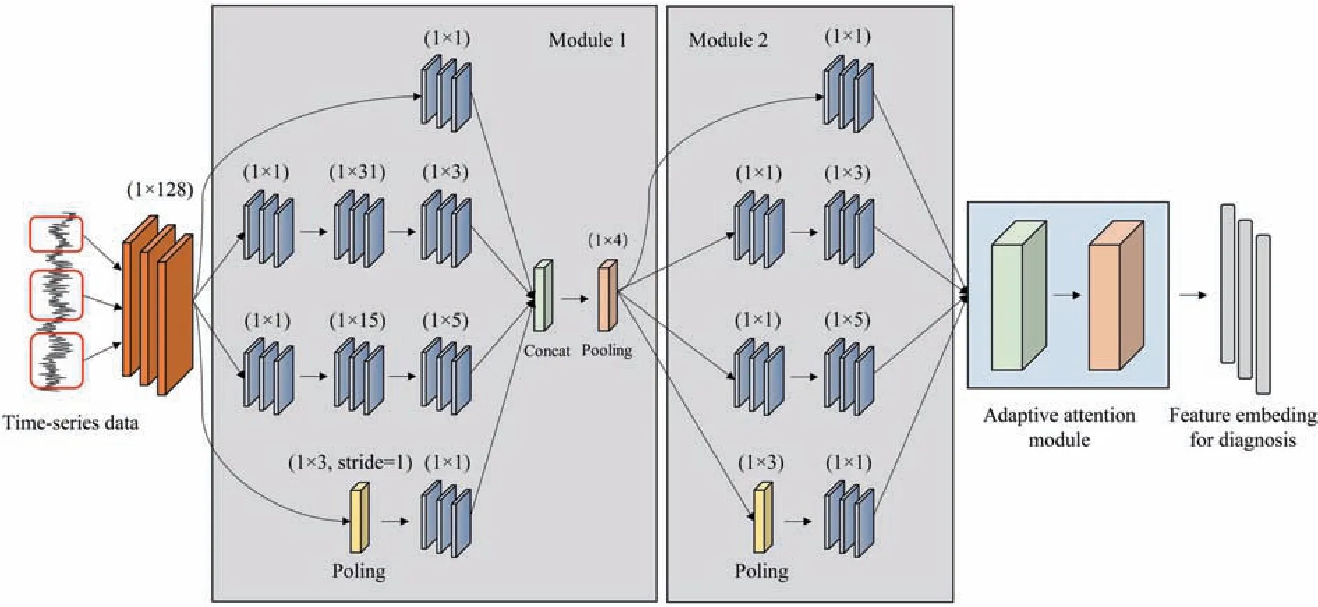
Fig.2.Illustration of the multiscale convolution architecture.

Fig.3.Adaptive channel attention.

where σ performs the sigmoid function,favepoolingandfmaxpoolinglaunch the average-pooling and max-pooling operations,andW′andWare the weight matrixes of MLP.

The feature mapF′output by the adaptive channel attention algorithm is presented in the following form:

where ⊗represents the element-wise multiplication.Based on the excitation mechanism,the original feature maps extracted from different kernel widths are weighted-fused to get the novel feature maps with adaptive information scales.

2.2.2.Adaptive spatial attention

Different regions of the feature maps correspond to various variable relations and fault type characteristics.The adaptive spatial attention algorithm is employed to concentrate on the local information weighting to highlight significate features.The module combines the advantage of multiscale convolutions to handle the targeted features from all receptive fields.Fig.4 displays the working procedure of adaptive spatial attention.Followed by the output of adaptive channel attention,the channel information is aggregated by two pooling operations to form the spatial context descriptorsThe average-pooled and max-pooled features across the respective channels are forwarded to be concatenated and convolved by the convolutions at different scales.Next,the features are fused via an element-wise summation which is formulated in (3).

whereciis the convolution operation of theith kernel size andnis the number of convolution branches.

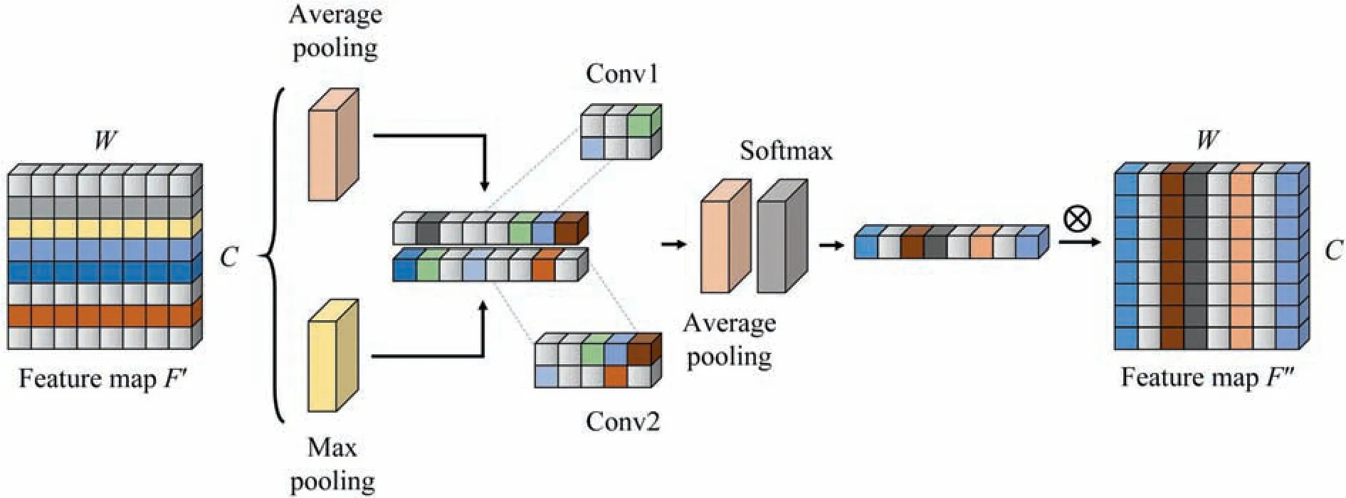
Fig.4.Adaptive spatial attention.

Average pooling is executed along the branch axis to generate spatial statistics ass∈R1×Land the softmax operator is followed close behind.The final spatial descriptorSis the compilation of each calculated element which is gained through the attention weights on various kernels.

Therefore,the final extracted feature map by adaptive spatial attention is computed asF′′.

To sum up,the adaptive attention module coalesced with the multiscale convolutions fulfills the adaptive feature fusion.The entire process of feature extraction and fusion is shown in Fig.5.Compared to the traditional attention mechanism,adaptive channel attention and adaptive spatial attention are embedded for automatic weighted mergence of multiscale features which boosts the feature learning of the AMCNN model.

2.3.Triplet loss optimization

The Triplet loss optimization is employed to achieve the generalization of fault features in different modes,which is first presented to learn better embeddings for face recognition in FaceNet model [35].It allows the model to upgrade to a deep embedding metric network and get a better classification performance.The illustration of the triplet loss optimization is presented in Fig.6.

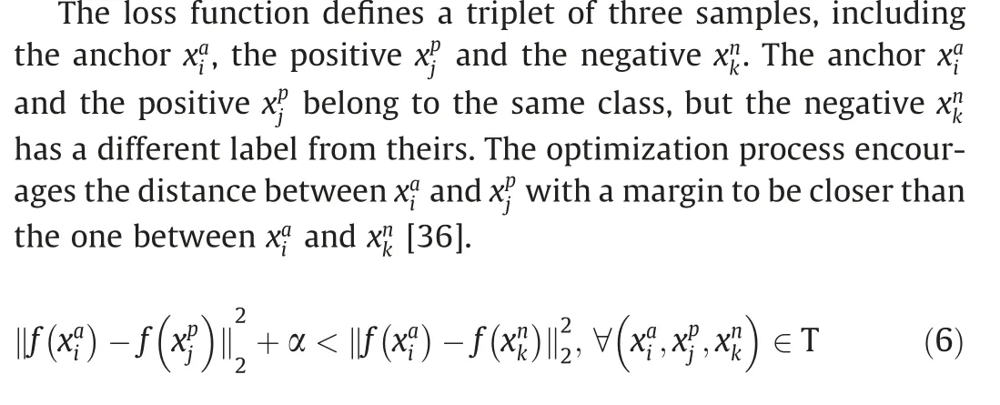
where α is a margin enforced between positive and negative pairs,T is the set of all possible triplets which has cardinalityN,f（·）represents the feature extractor in a deep network to obtain the feature embedding.

Fig.5.Feature extraction and fusion with multiscale convolutions and the adaptive attention module.

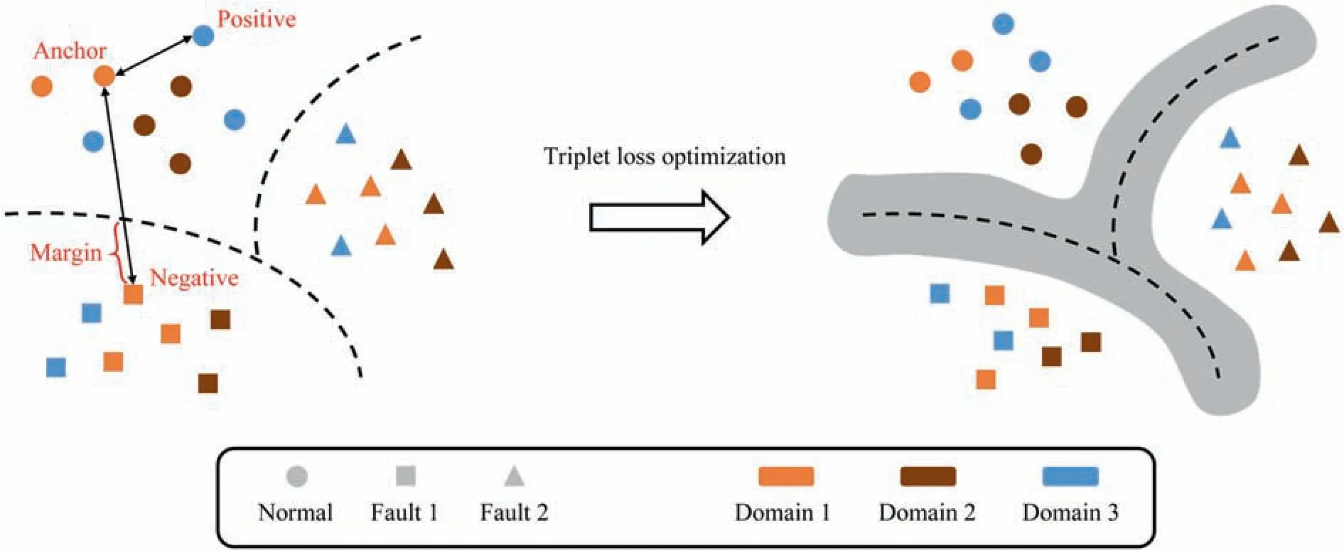
Fig.6.Illustration of triplet loss optimization.

It is crucial to select triplets that violate the triplet constraint in Eq.(7) to ensure fast convergence.Schroffet al.[35] define the triplets that fulfill Eq.(8) as easy triplets,and they do not need any optimization.Relatively speaking,hard triplets and semi-hard triplets are negative exemplars that are formulated as follows:

Semi-hard triplets are further away from the anchor than the positive exemplar,but the squared distance is still closer to the anchor-positive distance.These negatives lie inside the margin α.

As noted above,the triplet loss is designed to minimize the distance betweenandand maximize the distance betweenand.The formulation of the triplet loss is given as.

where [·]+means max（·,0 ）[37].Hard triplets and semi-hard triplets are selected to be optimized.With clustering the intrinsic distributions among multiple domains,the triplet loss optimization increases the discrimination of the diagnostic model and enhances its robustness under the multimode condition.

2.4.AMCNN-based fault diagnosis method

The detailed information of the proposed adaptive multiscale convolutional neural network model is unfolded in Fig.7.The multiscale feature extraction module operates on the input onedimensional data.The low-scale,mid-scale and high-scale kernels work in synergy.The adaptive attention module is embedded in the deep network which further improves the performance of feature selection.It adaptively pays more attention to the relevant information frames from the output of the convolutional layers.The selected features are input into two fully connected layers to recognize faulty conditions of the tasks.The classifier layer is constructed behind where softmax is utilized as activation function to output the probability of each class label.Triplet loss optimization is introduced to enhance the classification capability.The entire loss function of this network is defined in Eq.(10).

whereLcis the cross-entropy loss function of multi-classification,Ltis the optimized value of triplet loss,Lweightis the regularization of the model parameters to constrain the complexity of the network,λ and μ are the training coefficient set to 0.01 artificially.

The flowchart of the AMCNN-based fault diagnosis method is shown in Fig.8.The procedures are described in detail below.

Fig.7.Overview of the structure of the proposed AMCNN.

Fig.8.Framework of AMCNN-based fault diagnosis method.

The offline stage can be divided into the following steps:

Step 1: A training dataset that contains normal and faulty data is generated for model building.

Step 2:Normalize the data of each variable with mean and standard deviation with label information.

Step 3:The AMCNN model is constructed based on the training dataset.The model hyperparameters are adjusted with the experimental requirements and continuously optimized according to the training results.

Step 4:The trained model is tested with the validation dataset,and the monitoring performance of the classifier is tested.

Step 5:If the testing results are satisfactory,the model is saved and prepared for further application.Otherwise,the feature extraction module and the classification module should be modified and retrained.

The online stage can be divided into the following steps:

Step 1: The AMCNN model saved at the off-line stage is loaded and prepared for real-time fault diagnosis.

Step 2:The real-time process signals under the multimode condition are collected from the task system.

Step 3: Data normalization with the same mean and standard deviation as training proceeding.

Step 4: The time-series data from the same working mode or other domains is put into the loaded diagnostic model for feature extraction in the new observation and testing.

Step 5:The diagnosis results are output and the accurately recognized rate is calculated.

3.Case Studies

In this section,the fault diagnosis performance of the proposed AMCNN model is evaluated by a non-isothermal continuous stirred tank reactor(CSTR)simulation and the Tennessee Eastman process(TEP),where AMCNN is compared with two classical statistical models,least-squares support vector machine (LSSVM) [38] and random forest (RF) [39],and other popular deep learning models,including DCNN[25],stacked denoising autoencoders(SDAE)[19],and MSCNN [26] for ablation experiments.

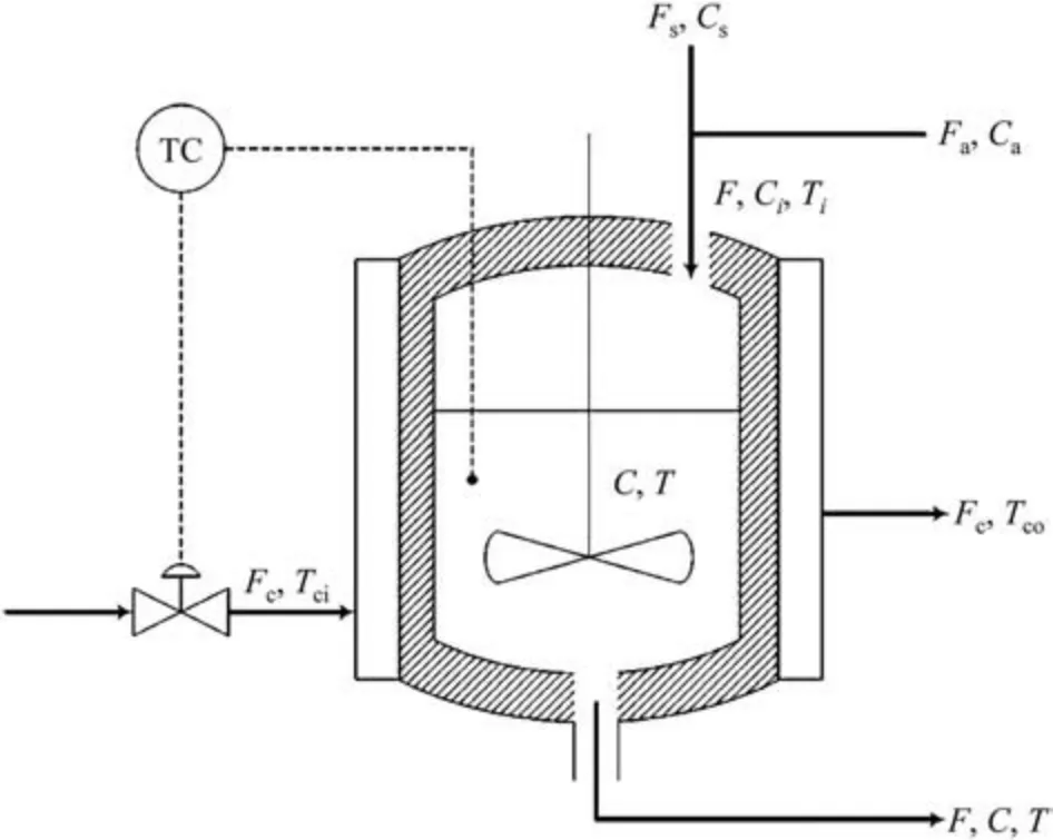
Fig.9.Process flow diagram of the CSTR system.

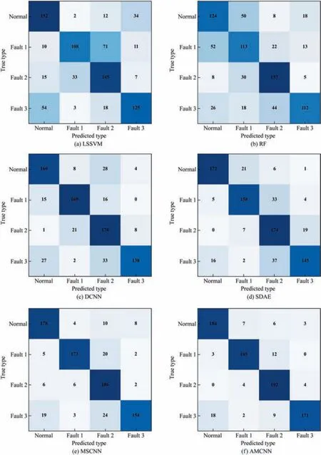
Fig.10.Diagnosis results by different methods for CSTR.

In order to represent the experimental results directly,the confusion matrix for theith class in multi-class classification tasks is defined as Table 1.The accurate diagnosis rate(ADR)is introduced in the following form:

Table 1 Confusion matrix for the ith class

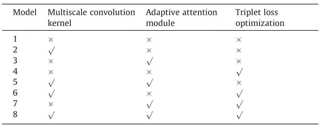
Table 2 Usage of different modules in the ablation experiment

Table 3 Comparison of the classification results of the ablation experiment

Table 4 Setting information of four modes in the CSTR simulation

ADR is a total classification accuracy of the fault diagnosis task which reflects the general performance of a model.The higher ADR is,the more accurately the model recognizes the fault type.

3.1.CSTR simulation

The AMCNN model is applied to the simulated non-isothermal CSTR system described by Yoon and MacGregor [40] and Choet al.[6].The reaction is the first order with the assumption that the reactor is well-mixed and the physical properties of the products are constant.The process flow diagram of the CSTR system isshown in Fig.9.The process has a feed stream which is the merged stream of the reactant A and the solvent S,a product stream,and a cooling water flow that controls the reaction temperature.The simulation system consists of the reaction component material balance and the energy balance,which are performed as follows:

whereVis the volume of reacting mixture,k0is the first-order reaction rate constant,Eis the activation energy,Ris the gas constant,ρ and ρcare the density of reacting mixture in the feed stream and coolant,cpandcpcare the specific heat capacity of the reacting mixture and coolant,ΔHrxnthe reaction enthalpy.

There are nine process variables collected by the sensors,including the inlet temperatureTi,the cooling water temperatureTci,the cooling water flowFc,the reaction temperatureT,the solvent flowFs,the reactant flowFa,the outlet concentrationC,the inlet concentrationsCaandCs.The simulation conditions are similar to Alcala and Qin [41].The setting information and the parameters are given in Appendix.Three scenarios of disturbances are introduced separately into the simulation system to describe the abnormal conditions:

(1) a step bias of the reaction temperatureTiby adding 1.5 K.

(2) a step bias of the inlet concentrationCaby adding 1.0 kmol·m-3.

(3) a ramp change of the inlet concentrationCaby making=0.1 kmol·m-3·min-1.

The simulations are performed under the normal and the three fault conditions in a certain mode called Mode 1.The variables are sampled every minute and the system is simulated for 400 min with each disturbance made att=151 min.200 samples containing 150 normal ones and 50 abnormal ones are used as the training dataset,while the last 200 samples are divided into the test dataset.

The confusion matrices of different fault diagnosis methods are shown in Fig.10.The results depict that the AMCNN model achieves the best diagnosis performance.The two traditional statistical models cannot determine the categories of failures accurately and the diagnosis results of the other deep learning models are worse than the proposed model.

According to the point of view of Choet al.[6],the first two faults are seen as simple faults which are caused by sensor biases and influence only one measurement heavily.Therefore,the above approaches diagnose the abnormality of CSTR simulation well in these scenarios.The third fault is a slow drift in the reaction kinetics.Catalyst poisoning leads to the exponential degradation of the reaction rate.It affects several other variables such as the output temperatureTand the cooling water flowFcso that it is regarded as a complex fault.On this occasion,AMCNN shows a pleasing result of fault identification while the other data-driven methods cannot recognize the fault type efficiently.

To further validate the optimal network architecture,the ablation experiment is applied based on the dataset mentioned above.The usage of different modules in the ablation experiment is displayed in Table 2.When the multiscale convolution kernels are not selected,the traditional convolution kernels will take replace.The comparison of the classification results is shown in Table 3,which is the overall ADR of all categories.The three core modules of AMCNN have a cooperative relationship and work together to achieve the effectiveness of the entire framework.

In order to verify the robustness of the AMCNN model under the multimode condition,four modes are set in the CSTR simulation as Xiaoet al.[42].The mode setting information is presented in Table 4.The experiments are conducted across different operating situations with domain transfer between discrepant datasets.In each working mode,all monitored measurements are captured in the normal condition and three abnormal conditions in the same way as above.The diagnosis results are presented in Table 5.It is observed that AMCNN identifies the faults more precisely than the other models and MSCNN takes second place which implies that the adaptive attention module enhances the classification ability of the network.

Table 5 ADR comparison of different methods under the multimode condition

The receiver operating characteristics (ROC) curve presents the model classification performance as a trade-off between selectivity and sensitivity.The false positive rate and the true positive rate are served as the axes of an ROC curve and the area under the curve is a quantitative way for classifier comparison.The model which gets the ROC curve closer to the upper left corner and the higher AUCvalue achieves the better diagnosis effect.Fig.11 demonstrates the ROC curves and the AUC values of AMCNN and MSCNN under the multimode experimental condition.The proposed AMCNN model proves its versatility for different working circumstances with data domains migration from the source mode to the unknown target mode.

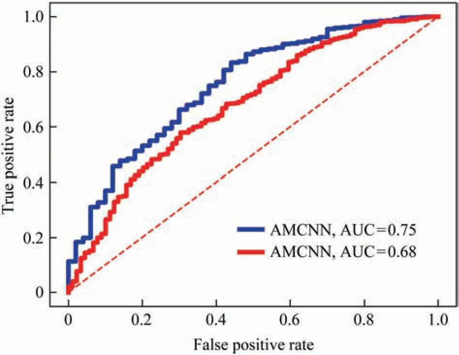
Fig.11.ROC curves and AUC values compared by AMCNN and MSCNN.

3.2.Tennessee Eastman process

The TEP which was first designed by Downs and Vogel[43]has been regarded as an industrial challenge for researchers in process monitoring.The revised version of the TEP is used in this experimental section which is available at https://depts.washington.edu/control/LARRY/TE/download.html [44].It is presented as a chemical process simulator with 52 variables including 41 measured variables and 11 manipulated variables under observation.The redundant manipulated variable XMV(12) representing the agitator speed is excluded which keeps constant during the simulation.There are 28 process disturbances programmed in the revised simulator which make the process operate on abnormal conditions.The first 20 types defined in Table 6 are selected for comparison with other algorithms.

The process consists of five unit operations: a reactor,a condenser,a vapor-liquid separator,a recycle compressor and a stripper.The schematic of the TEP model is shown as Fig.12.Two products are produced from four reactants with an inert and a byproduct involved.Except for the base case for initial setting,there are six modes of process operations at different product mass ratios or production rates.Mode 1 is utilized as a benchmark in the following experiments.

The data preparation and simulation process refers to[25].The measurements are generated on MATLAB/Simulink shown in Table 7.The sampling interval is set to 3 min.The model firstly runs for 500 h in the normal state with 10,000 normal sample matrices collected.For 20 different faulty states,the process simulation repeats for 10 times.The model runs for 50 h in each simulation with the specific disturbance introduced after the initial 10-hour normal running.Therefore,there are 40 h of simulation data and 800 fault sample matrices collected for every run of a fault type.It should be noted that the simulation can only last for 7 h after the disturbance IDV (6) is inserted because some variables will exceed the allowable limits.For normal data,80% of the sample matrices are randomly selected as the training set while the remaining as the testing set.For faulty data,eight runs of the simulation data are randomly chosen for training with the other two for testing.

The recognition rates of AMCNN are compared with the above mentioned diagnostic models in Table 8.For the overall performance of the models,AMCNN reaches the highest average accuracy which is 3.65% higher than MSCNN and 5.78% higher than DCNN.The corresponding recognition rates of 17 fault types are higher than 90%,and the proposed model displays the best diagnostic performance in 14 kinds of abnormal conditions.Considering the previous works,IDV(3) and IDV(16) make the diagnosis results unsatisfactory in some of the published models,but AMCNN overcomes these challenges.Fig.13 illustrates the confusion matrix of the proposed model’s diagnosis results,where the main diagonal numbers are the percentage of samples correctly identified and label 0 means the normal condition.As shown in the confusion matrix,IDV(9) and IDV(15) are still hard to recognize.The combined effect of the input disturbances and the internal control system makes the situation hard to be distinguished from the normal state and the other faulty states.The rest of the tested models perform better on some specific faults,such as RF on IDV(13),SDAE on IDV(17),and DCNN on IDV(10) and IDV(11).In general,AMCNN reveals its powerful performance in classification and extends the processing capability of traditional convolutional networks for time-series data.

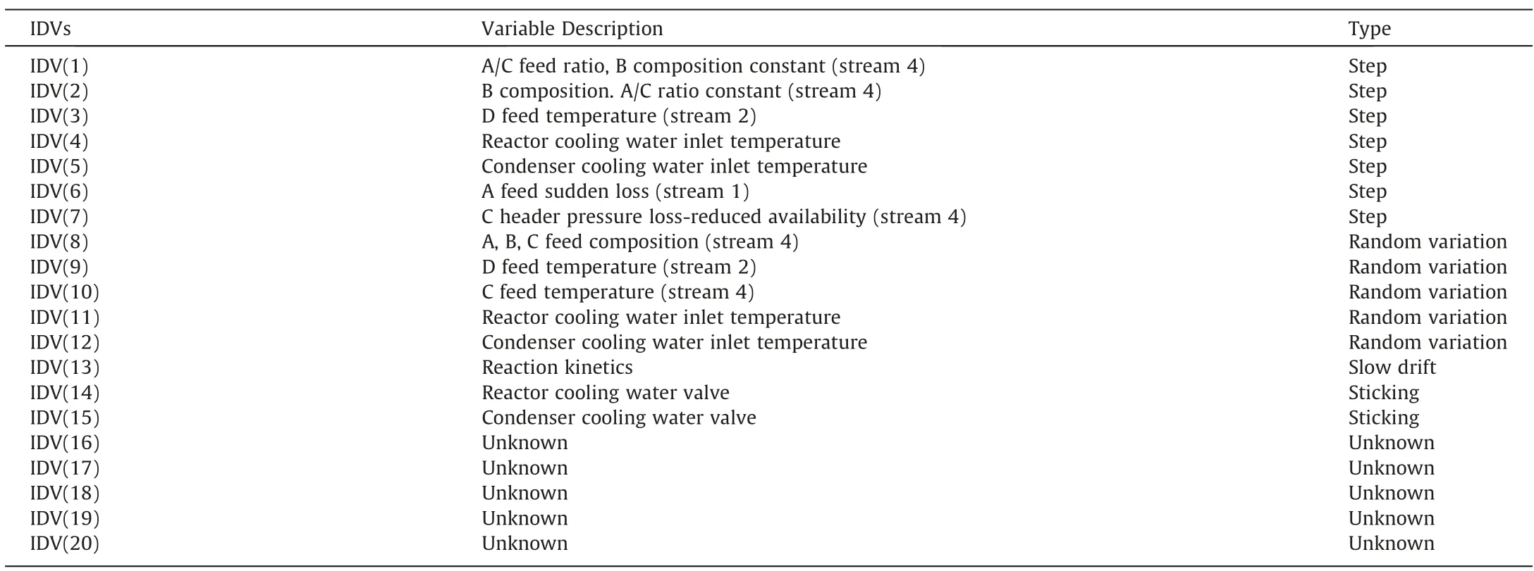
Table 6 Process disturbances in the TEP

Table 7 The sample matrices collected from the TEP for training and testing

Table 8 ADR comparison on the TEP

Fig.12.Schematic of the TEP.

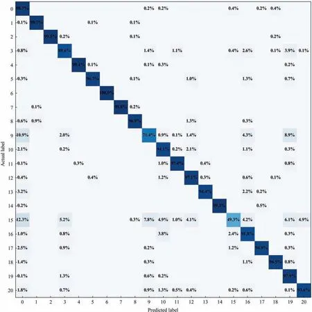
Fig.13.Recognition rates of AMCNN in a confusion matrix.

In order to demonstrate the generalizability of AMCNN in multimode fault diagnosis tasks,the other five different running modes are introduced as the experimental data.The descriptions of these working conditions are detailed in Table 9.The rules of the TEP simulation and data preparation are fulfilled in the same way.The training and testing sets are selected from mutually exclusive modes which indicates that the fault data of the source mode is applied to assist the diagnosis model training for the unseen target mode.When the simulation data of a certain mode is used for diagnosis,the data of the rest modes is used for training separately.Therefore,each of the methods to be tested undergoes a group of 30 pair experiments and then the comprehensive diagnosis rate is calculated to evaluate its performance.

Table 10 shows the overall ADR of the models involved in this paper.On account of the poor recognition precision of LSSVM,RF and SDAE,the detailed results of fault diagnosis for each mode pair are exhibited in Table 11 with only AMCNN,MSCNN and DCNN contrasted.It is observed that deep learning models are more robust than statistical models facing the industrial challenge of manufacturing mode switching.According to the compared outcomes,AMCNN still outperforms all the other models,certifyingthat the adaptive attention module and the triplet loss optimization achieve significant improvements on feature learning of the proposed model from process signals directly.The effectiveness of AMCNN under the multimode condition confirms that the features extracted at different scales can fully characterize the data distribution and the intrinsic interaction between multiple variables.The integrated model becomes more adaptive between the source mode and the target mode.

Table 9 Descriptions of six running modes of the TEP

Table 10 Overall ADR comparison on the TEP under the multimode condition

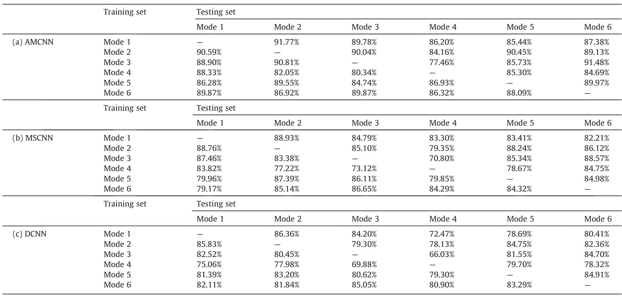
Table 11 Detailed results of fault diagnosis with AMCNN,MSCNN and DCNN

4.Conclusions

In this paper,an adaptive multiscale convolutional Neural Network (AMCNN) model is proposed for fault diagnosis of chemical processes.Different from the traditional deep CNN framework,the end-to-end learning model directly takes raw time-series data as input and captures multiscale features automatically.Adaptive attention mechanism constituted by channel-wise attention and spatial-wise attention stimulates key feature selection for classification across different working modes.Metric loss optimization through the triplet loss function facilitates the construction of generalized decision boundaries by narrowing the intra-class distance of features and expanding inter-class differences,which augments the discriminative capability of the network.The CSTR simulation and the TEP are utilized to highlight the applicability of the proposed model.AMCNN model creates higher-precision judgments on fault types compared with other commonly used diagnostic models no matter whether the process is under the multimode production situation.From the perspective of process safety,AMCNN can accurately recognize various types of faults in chemical processes and provide the basis of decision on the follow-up fault elimination.

Several issues also deserve further study in the future.First,AMCNN takes a little more time than the traditional CNN or statistical models for diagnosis due to the complexity of the model.It is a noteworthy task to make the model lightweight and accelerate the proceeding while maintaining its powerful identification accuracy.Subsequently,as a supervised diagnostic model,it is essential to further reduce the dependence on the labeled data.AMCNN is required to demonstrate its effectiveness with limited training data.Last but not least,the published fault diagnosis models including AMCNN still count on the knowledge of fault categories that have occurred before.These current models are likely to classify a brand new fault as an old type.A possible situation based on the application of AMCNN is to evaluate the contribution of each process variable or representative captured feature.The weight combination bestowed on the variables or features in the model is a symbol to define the attributes of the new fault.

Declaration of Competing Interest

The authors declare that they have no known competing financial interests or personal relationships that could have appeared to influence the work reported in this paper.

Acknowledgements

The authors gratefully acknowledge support from the National Science and Technology Innovation 2030 Major Project of the Ministry of Science and Technology of China(2018AAA0101605) and the National Natural Science Foundation of China (21878171).

Appendix.CSTR simulation parameters and initial conditions

The simulation parameters of the CSTR system areV=1 m3,ρ=106g·m-3,ρc=106g·m-3,E/R=8330.1 K,cp=1 cal·g-1·K-1,cpc=1 cal·g-1·K-1,b=0.5,k0=1010m3·kmol-1·min-1,a=1.678×106cal·min-1·K-1,ΔHrxn=-1.3 × 107cal·kmol-1.

The information of the temperature PI controller isKC=-1.5,TI=5.0.

The initial conditions for the simulation areTi=370.0 K,Tci=365.0 K,Fc=15 m3·min-1,T=368.25 K,Fs=0.9 m3·min-1,Fa=0.1 m3·min-1,C=0.8 kmol·m-3,Cs=0.1 kmol·m-3,Ca=19.1 kmol·m-3.

Measurement noises and disturbances are described asxt=φxt-1+σeet,xt,meas=xt+σmmt.Gaussian noise with small variance is added to the simulation,and the detailed setting information can be checked in [40].