
THE MAXIMIZATION OF THE ADMISSIBLE SAMPLING INTERVAL OF BOUNDARY PROPORTIONAL SAMPLED-DATA FEEDBACKS FOR STABILIZING PARABOLIC EQUATIONS
2022-11-27 05:45WANGXiangyuLIUHanbing
数学杂志 2022年3期
WANG Xiang-yu,LIU Han-bing
(School of Mathematics and Physics, China University of Geosciences, Wuhan 430074, China)
Abstract: In this paper,we study the problem of boundary sampled-data feedback stabilization for parabolic equations. By using modal decomposition, we show that there exists boundary proportional sampled-data feedback locally exponentially stabilize a class of parabolic equations,and the admissible sampling interval of this feedback is maximal among all feasible proportional sampled-data feedbacks.
Keywords: parabolic equations; sampled-data control; admissible sampling interval
1 Introduction
In this work, we study the following parabolic equation with boundary control

where Ω is a bounded and open domain of Rdwith a smooth boundary ∂Ω = Γ1∪Γ2, Γ1,Γ2being connected parts of ∂Ω, andnstands for unit outward normal on the boundary∂Ω. y0∈L2(Ω) is the initial data, and f is a nonlinear function defined on ¯Ω×R. The sampled-data controller u is applied on Γ1while Γ2is insulated. By sampled-data control,we mean that the control is a piecewise constant function in time. More exactly, it is of the form Here χ[ti,ti+1)is the characteristic function of interval [ti,ti+1) for i = 0,1,2,..., where 0 =t0<t1<···<ti<ti+1<···, with limi→∞ti=∞,are sampling time instants,the positive numbers Ti=ti+1-ti, (i=0,1,2,···) are called the sampling intervals.

Sampled-data feedback stabilization is a well-studied topic for finite dimensional systems due to the fact that modern control systems employ digital technology for the implementation of the controller. However, for sampled data feedback stabilization of infinite dimensional systems, the research results are relatively few.
To stabilize the infinite dimensional systems by sampled-data feedback control,most of existed works applied directly the feedback which works for the continuous-time case (see[1-4]). It was shown that the continuous-time stabilizing feedback can stabilize the sampleddata system when the sampling intervals are small enough. However, the requirement that sampling intervals are sufficiently small is not reasonable from two perspectives: smaller sampling intervals require faster,newer and more expensive hardware;performing all control computations might not be feasible,when the sampling interval is too small(see Section 1.2 in[5]). Recently, the second author and collaborators considered the stabilization of parabolic equations with periodic sampled-data control, and developed methods to design feedback laws for any known sampling period (see [6, 7]).
For the case when the sampling intervals are variable and uncertain,usually it is unable to design a feedback to stabilize the system for arbitrary sampling intervals. What we can do is try to find a feedback such that its admissible sampling interval is largest. By admissible sampling interval of a sampled-data feedback, we mean that for all sampling instants whose sampling intervals are less than or equal to it, the feedback stabilizes the equation (It’s mathematical definition will be given in Definition 2.1). In general, it is very difficult and almost impossible to find such an optimal one from all feedbacks. In this work, we consider a class of special feedbacks, i.e. the proportional feedbacks. Such kind of feedback controls are simple, and easy to be implemented, and they have been used by V.Barbu and later on developed by I. Munteanu to stabilize various systems under continuous-time boundary feedback control in[8-10]. Giving the decay rate and the lower bound of sampling intervals,under the assumption proposed by V.Barbu, we shall construct an explicit sampled-data feedback to exponentially stabilize the parabolic equations, and the admissible sampling interval of the feedback is maximal among all feasible proportional feedbacks.
The main novelties of this work can be summarized as following: Firstly,compared with[6] and [7], we consider in this work the case that the sampling intervals are variable and uncertain, and the feedbacks do not depend on the sampling intervals but only the lower bound of these intervals. Secondly, comparing with existed literatures, this work makes the first attempt to achieve the largest admissible sampling interval.
The rest of this paper is organized as follows. In Section 2, we shall construct the feedback control, and prove that it stabilizes the linearized equation and it maximizes the admissible sampling interval. In Section 3, we will show the feedback control constructed in Section 2 also locally exponentially stabilizes the semilinear parabolic equations.
2 Stabilization of the Linearized Equation
2.1 The Linearization of Semilinear Parabolic Equation and Notations
The equilibrium solutions ye∈C2(¯Ω) is any solution to the equation

2.2 The Stabilization of the Linearized Equation

In practice,the sampling intervals should not tend to zero. Hence,we make the following assumption throughout this work:
(Hs) Ti=ti+1-ti≥T, i=0,1,2,··· , where T >0 is given.
We introduce firstly the proportional feedbacks we shall consider. Let

where F ∈F, can be written as

Let ρ be given by (2.3) and T be given in (Hs). We give the notion of the admissible sampling interval of a feedback.
Definition 2.1 (i) We call F ∈F a feasible feedback if F ∈Fρ, where Fρis given by


Remark 2.2 Arbitrarily giving T <TF, from above definition, we see that, ∀{ti}∞i=0satisfying Ti= ti+1-ti∈[T,T], the system (2.6) can be exponentially stabilized by the boundary sampled-data feedback F.
Then the problem we shall study in this section can be formulated as follows.
Problem (PT,ρ) Find the optimal feedback F*∈Fρ, such that the feedback F*maximizes the admissible sampling interval, that is

The following theorem contains the main results of this section, which give the optimal value and the optimal solution of the Problem (PT,ρ).
Theorem 2.3 Assume~y0∈L2(Ω),under the assumptions(Hn)and(Hs),the following results are true:

(iii) The key point to solve Problem (PT,ρ) can be explained roughly as follows: We firstly reduce the stabilization of system(2.6)to solve the following inequalities with respect to γj, j =1,2,··· ,N,


(iv) The above design applies as well to equation (2.6) with homogeneous Dirichlet condition on Γ2and Dirichlet actuation on Γ1, that is y = u on Γ1; y = 0 on Γ2, or to the Neumann boundary control, but we omit the details.
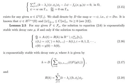
To prove Theorem 2.3, we shall use the Dirichlet map to lift the boundary condition,and transfer the nonhomogeneous problem to a homogeneous one. This preliminary result will be presented in Lemma 2.5, and it will not only be used in the proof of Theorem 2.3,but also useful for the proof of stabilization for the nonlinear equation (1.1).
To state Lemma 2.5, we need to introduce the so-called Dirichlet map. It is well-known that for sufficiently large k >0, the solution to the equation
Proof We will divide the proof into two steps.
Step 1 We prove the relation of y and z. We will find the relationship between y and z by lifting the boundary condition for equation (2.6).
Setting ~z(t,x)=y(t,x)-h(t,x), by (2.6), (2.15) and (2.17), it is not difficult to prove that ~z satisfies exactly equation (2.16) (The second identity of (2.16) holds because y is continuous). Hence, ~z(t,x)=z(t,x) and

On the other hand, suppose that ∃C5>0,ρ >0, s.t. ‖y(t)‖ ≤C5e-ρt‖y(0)‖. For the same reason, one can obtain that ∃C >0, s.t. ‖z(t)‖≤Ce-ρt‖z(0)‖.
This completes the proof of Lemma 2.5.
Now, we give the proof of Theorem 2.3.


3 Stabilization of Nonlinear Equation

For the stabilization of the semilinear parabolic equation (1.1), we have the following result.

The proof of this theorem is similar to that of Theorem 3.1 in [6]. Therefore, we omit the proof here.

- 数学杂志的其它文章
- RESEARCH ANNOUNCEMENTS ON “STRUCTURAL STABILITY OF TRANSONIC SHOCK FLOWS WITH EXTERNAL FORCE”
- ORDER STATISTICS OF MULTIVARIATE ERLANG MIXTURES WITH APPLICATION IN MULTIPLE LIFETIME THEORY
- STRONG ATOMIC DECOMPOSITIONS OF TWO-PARAMETER B-VALUED WEAK ORLICZ STRONG MARTINGALE SPACES
- 分数布朗单驱动的随机微分方程的传输不等式
- LBRAGIMOV-GADJIEV-DURRMEYER 算子在ORLICZ空间内的逼近性质
- 基于BFGS修正的HSDY 混合共轭梯度