The Quasar Candidate Catalogs of DESI Legacy Imaging Survey Data Release 9
Zizhao He and Nan Li
1 Key Laboratory of Space Astronomy and Technology, National Astronomical Observatories, Beijing 100101, China; nan.li@nao.cas.cn
2 School of Astronomy and Space Science, University of Chinese Academy of Sciences, Beijing 100049, China
Abstract Quasars can be used to measure baryon acoustic oscillations at high redshift,which are considered as direct tracers of the most distant large-scale structures in the universe. It is fundamental to select quasars from observations before implementing the above research.This work focuses on creating a catalog of quasar candidates based on photometric data to provide primary priors for further object classification with spectroscopic data in the future,such as the Dark Energy Spectroscopic Instrument (DESI) Survey. We adopt a machine learning algorithm (Random Forest, RF) for quasar identification.The training set includes 651,073 positives and 1,227,172 negatives,in which the photometric information are from DESI Legacy Imaging Surveys(DESI-LIS)and Wide-field Infrared Survey Explore(WISE),and the labels are from a database of spectroscopically confirmed quasars based on Sloan Digital Sky Survey and the Set of Identifications& Measurements and Bibliography for Astronomical Data. The trained RF model is applied to point-like sources in DESI-LIS Data Release 9.To quantify the classifier’s performance,we also inject a testing set into the to-be-applied data.Eventually, we obtained 1,953,932 Grade-A quasar candidates and 22,486,884 Grade-B quasar candidates out of 425,540,269 sources (~5.7%). The catalog covers ~99% of quasars in the to-be-applied data by evaluating the completeness of the classification on the testing set.The statistical properties of the candidates agree with that given by the method of color-cut selection. Our catalog can intensely decrease the workload for confirming quasars with the upcoming DESI data by eliminating enormous non-quasars but remaining high completeness.All data in this paper are publicly available online.
Key words: (galaxies:) quasars: general – catalogs – methods: statistical
1. Introduction
The discovery of quasars,also known as quasi-stellar objects(QSOs), is one of the four significant findings that have been made in astronomy in the 60 s of last century (Schmidt 1963;Kellermann 2014).QSOs are extremely luminous active galactic nuclei (Osterbrock 1989; Urry & Padovani 1995; Dunlop et al.2003; Croton et al. 2006, AGN) powered by accretion onto supermassive black holes at the centers of galaxies, and their typical luminosity is 1042to 1048erg s-1(Shen et al.2020)at the redshift from 0.1 to 7(Antonucci 1993).The emission of QSOs can significantly outshine their host galaxies, and their emitting regions are too small to resolve even for the nearest ones.Hence,QSOs are always considered point-like sources, which mimic faint blue stars in optical bands. However, they are ~2 mag brighter in the near-infrared at all redshifts than stars of similar optical magnitudes and colors, leading to a neat way to discriminate QSOs from stars (Ross et al. 2012; Myers et al.2015; Yèche et al. 2020).
The nature of QSOs has been investigated widely and thoroughly in the past decades by using tons of corresponding observations.Consequently,QSOs are used to study astrophysical problems in various fields.For instance,the spectrum of QSOs is a powerful tracer of the formation and evolution of black holes,the spins of black holes, and the co-evolution of black holes and host galaxies (Kormendy & Richstone 1995; Silk & Rees 1998;Kaspi et al. 2000; Di Matteo et al. 2005; Springel et al. 2005;Kormendy&Ho 2013;Chen 2021;Valentini et al.2021);taking advantage of microlensing, astronomers study the feature of accretion disks with the light curves of QSOs (Agol &Krolik 1999;Morgan et al.2010;Blackburne et al.2011;Dexter& Agol 2011); the absorption lines of quasars are unique tracers of the interstellar media along the line of sight (Scaringi et al.2009;Hall et al.2013;Chen et al.2020;Mishra et al.2021;Zabl et al. 2021). Besides, high-redshift quasars are valuable for understanding the reionization of the universe and the formation of galaxies(McLure&Jarvis 2002;Wang et al.2019;Lupi et al.2021). Statistically, the spatial distribution of quasars reflects the baryon acoustic oscillations(BAOs,e.g.,Zhao et al.2019,for an introduction) and in turn the large-scale structure of the universe(Dawson et al.2013;Font-Ribera et al.2014;Delubac et al.2015;Alam et al. 2021; Merz et al. 2021). Expectedly, with the nextgeneration large-scale surveys coming,an unprecedented data set of QSOs brings an unparalleled opportunity to trigger a revolution in these fields.
Mining QSOs from enormous data sets is crucial for carrying out the studies mentioned above, and plenty of progress has been made. The Palomar-Green Bright Quasar Survey (BQS,Schmidt & Green 1983) discovered more than 100 quasars.The Large Bright Quasar Survey (LBQS, Hewett et al. 1995)discovered more than 1000. The 2° Field Quasar Redshift Survey(2QZ,Croom et al.2004)discovered about 23,000.The Large Sky Area Multi-object Fiber Spectroscopic Telescope(LAMOST,Dong et al.2018)discovered more than 20,000.At the moment,the largest confirmed quasar catalog is from Sloan Digital Sky Survey Data Release 16 (SDSS DR16, Blanton et al. 2017; Lyke et al. 2020), which contains 750,414 spectrally confirmed quasars. Nevertheless, to implement confirming QSOs with spectrums, one must create a sample of QSO candidates using or even combining various types of data other than spectroscopy.For instance,photometry data can be used to select QSO candidates according to the features of QSOs, such as the ultraviolet excess, infrared excess, and the light variation(Shen et al.2011);astrometry data kicks out the objects with high proper motion in the Milky Way (Fu et al.2021); and radio and X-ray data are valuable complements(Bisogni et al. 2021).
The Dark Energy Spectroscopic Instrument (DESI,3https://www.desi.lbl.gov/Levi et al. 2013; DESI Collaboration et al. 2016) is a spectral telescope that is located at Kitt Peak National Observatory(KNPO). It is a Mayall telescope with a four-meter-aperture primary mirror. It will target about 30 million pre-selected galaxies across ~14,000 square degree sky. It is important for the discovery of more quasar because of its large sky coverage,good image quality and depth (compared to SDSS, York et al.2000),and because it can provide spectrum.However,the QSO candidates are needed for further conforming the QSOs.Hence,we acquire the QSO candidates from the photometry catalog of DESI Legacy Imaging Survey (DESI-LIS).
In this work,to create a catalog of QSO candidates for DESI,we adopt a machine learning(ML)technology named Random Forest (RF) and apply it to photometry data from DESI-LIS because its efficiency, flexibility, and accuracy have been intensively proved previously (e.g., Viquar et al. 2018; Bai et al. 2019; Clarke et al. 2020; Guarneri et al. 2021), in particular, Bai et al. (2019) demonstrates that RF is the most efficient and reliable one among several methods in dealing with quasar-star-galaxy classification. The training and validation sets are built upon the spectra data from SDSS eBOSS(extended Baryon Oscillation Spectroscopic Survey, Dawson et al.2016)DR16 and the photometry data from WISE4https://irsa.ipac.caltech.edu/Missions/wise.html(Widefield Infrared Survey Explorer, Wrigh et al. 2010) and DESILIS, labels are generated based on the database of SIMBAD5http://simbad.u-strasbg.fr/(the Set of Identifications, Measurements and Bibliography for Astronomical Data, Wenger et al. 2000). To evaluate the completeness, accuracy, and purity of identifying QSOs candidates from the photometry data of point-like sources in DESI-LIS and WISE,we inject a testing set that mimics to-beapplied data in magnitude and color space. Later, the trained model is applied to point-like sources in DESI-LIS, and the quasar candidate catalogs are acquired. Finally, we compare our results to those of the color-cut selection approach for cross-validation, and they match well. For the convenience of other researchers, we make all the data in this paper publicly available online.6https://github.com/EigenHermit/he-li2021
The paper is organized as follows. The construction of the data sets used in this paper is presented in Section 2.Section 3 introduces the details of the methods for detecting QSOs adopted in this study. We then show the results in Section 4.Finally, Section 5 delivers the discussion and conclusions. In this paper, a fiducial cosmological model with Ωm=0.26,ΩDE=0.74, h=0.72, w0=-1 and wa=0 is adopted. The cosmology is the same as the one adopted in Oguri&Marshall(2010, OM10 hereafter).
2. Data sets
The data sets adopted in this work include DESI-LIS,WISE,SDSS eBOSS DR16,and SIMBAD.The training set combines photometry data from DESI-LIS and WISE, while the labels are from the confirmed QSO catalog from SDSS eBOSS DR16 and SIMBAD.The validation set is extracted from training set.To evaluate the performance of the classification of QSO candidates, we also build a testing set with the SIMBAD database and eBOSS data set. Introduction to the above data sets and details of the construction of training and testing sets are described below.
2.1. DESI-LIS, WISE, eBOSS, SIMBAD
DESI-LIS and WISE—DESI-LIS7https://www.legacysurvey.org/(Dey et al. 2019, DESILIS) contains Dark Energy Camera Legacy Surveys (DECaLS8https://www.legacysurvey.org/decamls/), Beijing-Arizona Sky Survey (BASS9https://www.legacysurvey.org/bass/) and Mayall zband Legacy Survey (MzLS10https://www.legacysurvey.org/mzls/), covering ~14,000 deg2of the extra-galactic sky in three optical bands (g, r, and z). Notably,DESI-LIS DR9 also includes four mid-infrared bands (at 3.4,4.6, 12, and 22 μm, corresponding to W1, W2, W3 and W4 respectively) observed by WISE.11http://wise.ssl.berkeley.edu/index.htmlWe adopt the photometry information in g, r, z, W1, W2 bands from the above data sets to search for the quasar candidates from 425,540,269 point-like sources in DESI-LIS DR9 catalog12https://www.legacysurvey.org/dr9/).
SDSS eBOSS DR16—The Sloan Digital Sky Survey(SDSS,see, e.g., York et al. 2000, for more details) is a major multispectral imaging and spectroscopic redshift survey and has a long-running history of more than 20 yr. The eBOSS(grounded upon SDSS-IV, Blanton et al. 2017) is an extended project of BOSS (Baryon Oscillation Spectroscopic Survey,grounded upon SDSS-III,Eisenstein et al.2011;Dawson et al.2013), which maps the LRGs (luminous red galaxies, Zhou et al. 2020; Fortuna et al. 2021) and quasars to determine the characteristic scale of BAOs imprinted at the large-scale structure. eBOSS covers a broader range of redshifts than that of BOSS.Based on the Data Release 16 of eBOSS,Lyke et al.(2020) publishes a catalog containing 750,414 quasars(DR16Q, hereafter), which is the largest catalog of quasars confirmed spectroscopically. We employ the classification labels from eBOSS DR16 to construct the part of positives in training and testing sets.
SIMBAD—SIMBAD is a comprehensive database that collects information on astronomical objects, such as types,fluxes, proper motion, etc., maintained by the Centre de données astronomiques de Strasbourg (CDS). To date,SIMBAD includes 11,953,504 objects, ~50% of them are stars (Paturel et al. 2003; Zuckerman et al. 2003; Cayrel et al.2004), and the others are non-stellar objects like AGNs,starburst galaxies, emission-line galaxies (Fu et al. 2021). The types of astronomical objects13http://simbad.u-strasbg.fr/simbad/sim-display?data=otypesin SIMBAD are derived from physical characteristics (Mickaelian et al. 2006; Małek et al.2010), and the astronomical objects with uncertain physical types are marked as “XX_Candidate” or “Possible_XX”, e.g.,“AGN_Candidate”. In addition, “main_type” and “other_types” are given in SIMBAD to deal with the situations in which different studies suggest different types of the same object.We use the non-QSOs data in SIMBAD to build the part of negatives in training and testing sets.
2.2. Training and Testing Data sets
The training and testing sets comprise photometry information and labels, where the photometry is from DESI-LIS and WISE, and the labels are from eBOSS DR16 and SIMBAD,respectively. To avoid the problem of overfitting, we extract a subset from the training set for creating a validation set.Notably, the testing set is organized for mimicking the to-beapplied data set to estimate the classification performance using our method.
Parent Samples—We first make two parent samples (hereafter, S1 and S2) to separately prepare the positives and negatives in training and testing sets. For S1, we first obtain 745,417 QSOs14https://www.legacysurvey.org/dr9/files/#survey-dr9-region-dr16qv4-fitsby combining the photometry in DESI-LIS and labels in DR16Q via cross-matching the catalogs ofDESI-LIS and DR16Q. Then, we clean the cross-matched catalog by selecting point-like sources in DESI-LIS (i.e.,classified as PSFs)that having all five-bands(g,r,z,W1,W2)detections. S1 holds 655,017 QSOs at last. Similarly, S2 is acquired by combining photometry in DESI-LIS and the classification labels in SIMBAD, and the cross-match between SIMBAD and DESI-LIS PSFs is executed. Besides, we clean the 1,993,373 sources obtained through the above procedure according to the “main_type” in SIMBAD. Details are listed below:
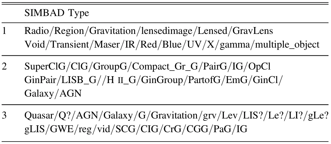
Table 1 The Types of Objects that we Abandon when Build the Training and Testing Set
1. The sources labeled as quasars are abandoned.
2. The sources classified by their SEDs (Spectral Energy Distributions, see e.g., Richards et al. (2006), for an introduction), region, numbers, time-domain characteristics and the ones with gravitational lensing effect are eliminated. Therefore, the types listed in the first line of Table 1 are excluded.
3. The sources that have uncertain physics types are discarded, i.e., we exclude all the sources that have“Candidate”, “Possible”, “?”, or “Unknown” in their“main_type”.
4. The sources classified as AGN and the types that relate to galaxies are excluded. Therefore, the sources have the labels listed in the second line of Table 1 are discarded. Although we only use point-like sources in DESI, some galaxies are still involved in DESI-LIS PSFs because extremely compact galaxies and the highdensity regions in large galaxies might be classified as point sources.
5. The “LINER”, “Blazar”, “Seyfert” and “BLLac” are cleaned because they mimic the color of the quasars(Peters et al. 2015).
After these operations, we further take care of the information given in “other_types”. We remove the sources that have the labels listed in the third line of Table 1. At the end, there are 1,363,030 non-QSOs left from 1,993,373 sources. Note that 99.85% of non-QSOs are stars, and the rests have non-stellar features such as “H II (ionized) region”(0.11%)and“Emission Object”(0.02%).Details of the catalog of negatives are available online.15
Testing Set—The testing set are constructed by selecting objects in S1 and S2 according to the distributions of magnitudes of QSOs in DESI-LIS modeled by a typical luminosity function (LF, hereafter) and an SED (Bianchini et al. 2019) because the distributions of QSO and non-QSO in testing set should be similar to the corresponding ones of DESI-LIS if we plan to evaluate the classification performance with the testing set.The LF is double power-law as is modeled in OM10:
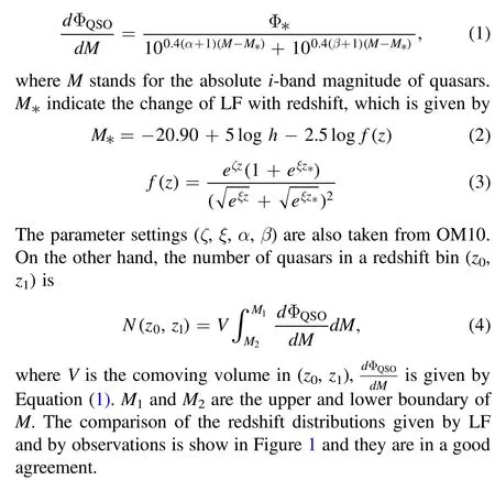

We further predict the magnitude distributions of g, r, zbands using a typical SED(Bianchini et al.2019)based on the i-band magnitude distribution of QSOs acquired above.According to the predicted distributions of g, r, z-bands, the W1, W2 is directly taken from 3944 quasars in S1. The W1,W2 cannot be calculated merely based on SED because the host galaxies of QSOs contribute to the total fluxes considerably in W1, W2 bands (Li et al. 2021). Thus, the 10,000 mock quasars form the positives in the testing set, and the distributions are shown in Figure 2.
Moreover, we select the non-QSOs from S2 to construct the negative part of the testing set. The criterion is that we find such non-QSOs to make the overall distributions(testing QSOs+ non-QSOs) similar to the overall distributions of DESI-LIS PSFs. The testing set contains 990,000 non-quasars (135,858 individual ones). The comparisons in magnitude and color spaces between DESI-LIS PSFs and the testing set are shown in Figure 3.In the space of all 15d colors,the twos show a good agreement and are particularly good in the color space (the mean and stranded deviation differences are less than 1%). In magnitude space, however, the testing set is slightly brighter than DESI-LIS PSFs due to the selection effect of SIMBAD.
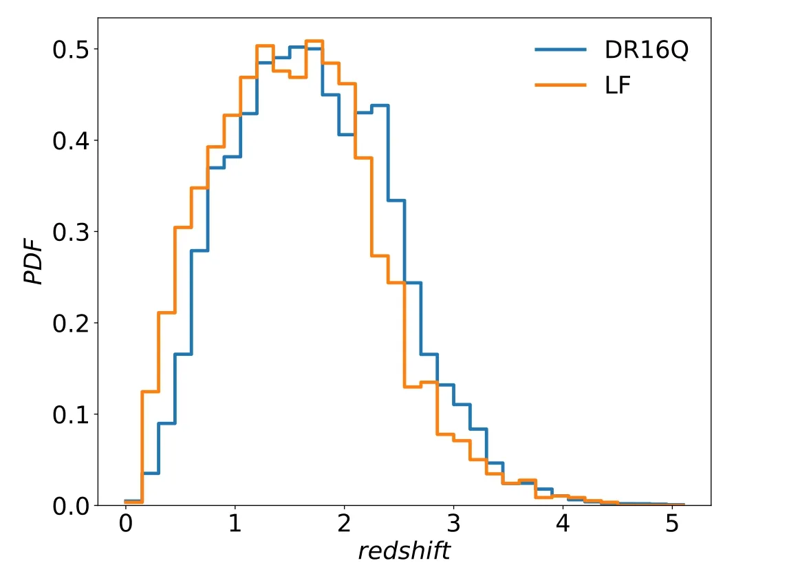
Figure 1. The comparison of redshfit distributions. The orange one is calculated by (1). The blue one is from DR16Q.
Above all, the testing set contains 100,000 sources, 1%(Page 2001)of them are quasars,built upon 3944 quasars in S1 and 135,858 non-quasars in S2.
Training Set—Except for the sources in the testing set, the rests in S1 and S2 comprise the training set.Explicitly,there are 651,073 positives and 1,227,172 negatives in the training set,and the distributions of quasars in the training set are shown in Figure 4.
3. Methodology
The primary approach for identifying QSO candidates is constructed upon RF in this work. The evaluation metrics for the outcomes include completeness, accuracy, and area under the receiver operating characteristic(ROC)curve(AUC).Also,we create a baseline for the identification of QSO candidates using the traditional color-cut selection method for crossvalidation.
3.1. Random Forest
RF is a mature ML algorithm and has been widely employed in astronomy. RF was first proposed and named “random decision forests” by Ho (1995), then improved and renamed“random forests” by Breiman (2001). The basic workflow of RF is that: (1) randomly segments the input data; (2) trains a group of decision tree models (Dobra 2018) with the segmented data separately; (3) gives the final judgments by combining the outputs of all decision trees.Breiman(2001)has suggested that RF compares favorably to AdaBoost(Freund&Schapire 1996)but it is more robust on missing and unbalanced data, and performs well on multi-dimension data.
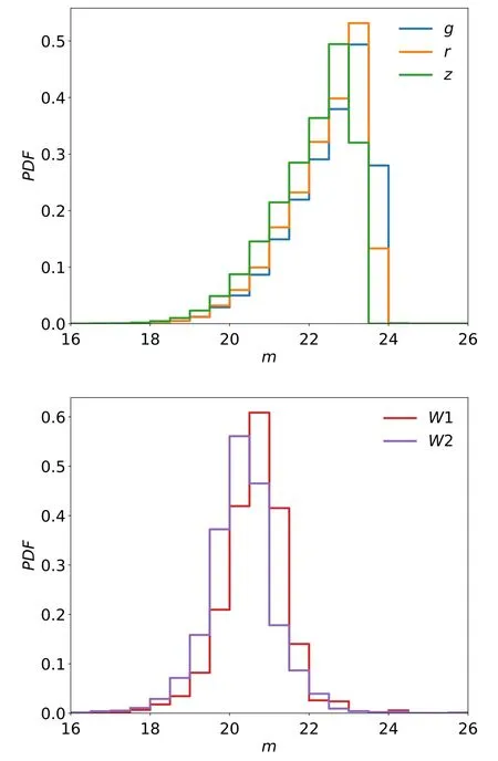
Figure 2.The distributions of g,r,z,W1,W2 of the quasars in the testing set.
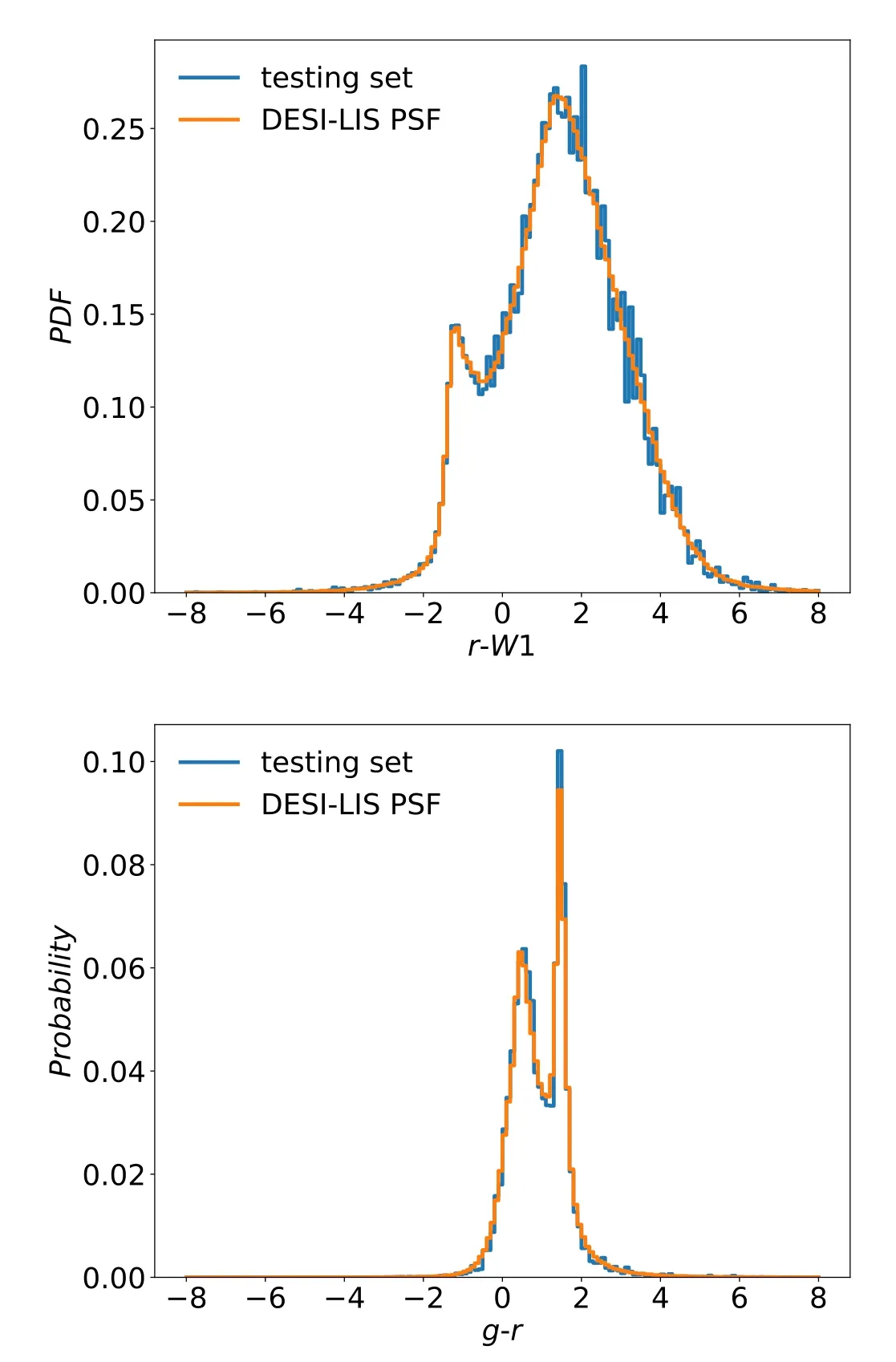
Figure 3. The comparisons between the testing set and DESI-LIS PSFs. The upper is in color space while the lower is in magnitude space.
In particular, when dealing with the classification of stargalaxy-quasar with photometry, Bai et al. (2019) presents the superiority of RF over K-Nearest Neighbor(Altman 1992)and Support Vector Machine (Cristianini & Ricci 2008) by implementing a comprehensively comparative investigation,which inspires us to choose RF for our purpose.


3.2. Color-cut Selection
The color-cut selection (in g-z versus grz-W space,following Yèche et al. 2020) is performed to validate the candidates that selected by RF model, which is a widely used method for selecting quasars with photometry data (see e.g.,Warren et al. 1991; Croom et al. 2004; Richards et al. 2005;Morganson et al. 2014, for the applications) because the magnitude of quasars in the UV band is brighter than normal stars and galaxies(Elvis et al.1994)comparing to the stars that have similar magnitudes in optical bands. QSOs are also roughly two magnitudes brighter in the near-infrared bands across a wide redshift range(Peters et al.2015).Above all,we slightly update the strategies of the color-cut selection procedure in Yèche et al. (2020), and create a QSOs candidate catalog for cross-validating with the results given by the RF model.Details of selection criteria are listed in Table 2,and the definitions are:
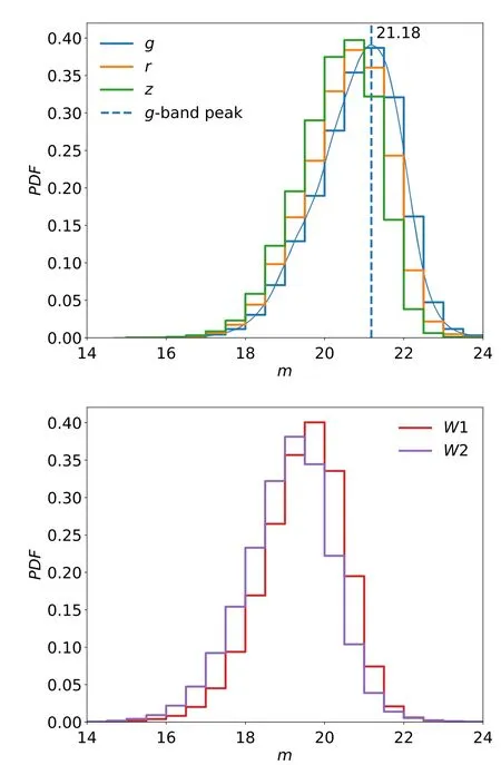
Figure 4.The distributions of g,r,z,W1,W2 of the quasars in the training set.The g-band peak magnitude is shown by the vertical dashed line, which is determined by a kernel density estimate plot (blue solid curve) that gotten by kdeplot in seaborn package with the default Gaussian kernel and binwidth=0.5.

The first four criteria in Table 2 are directly taken from Yèche et al. (2020) while the last one is designed to further limit the samples by taking advantage of the aforementioned infrared excess.We note that we use depth limit(g=22.7,similar with Yèche et al. 2020) in this color-cut selection.

Table 2 The Selection Conditions that used in Color-cut Selection (Detailed at Section 3.2)
3.3. Evaluation Metrics
Completeness, accuracy, and AUC are quintessential classification metrics, which measure the performance of classification models from various angles. The three quantities can be calculated by combining True Positives (TP), False Positives(FP),True Negatives(TN),and False Negatives(FN)in different forms. Specifically, completeness is given by

meaning the percentage of quasars in the testing set that can be correctly picked out; accuracy is given by

standing for how well the identification of quasars/non-quasars is;purity is used to assess how much non-quasar contamination in the quasar candidate catalogs, which is defined as

AUC is the area under the ROC (Fawcett 2006), showing the performance of the classification at all classification thresholds by plotting False Positive Rate(FPR)versus True Positive Rate(TPR), defined as

AUC represents the overall performance of identification results.
4. Results
In results of applying our classifier trained by the training set given in Section 2.2 to DESI-LIS point-like sources(Section 2.1), we accomplish a catalog of quasar candidates,detailed in Section 4.1. Then, we cross-validate the catalog with the results obtained via color-cut selection method (see Section 3.2), and the details are shown in Section 4.2.
4.1. Quasar Candidate Catalogs
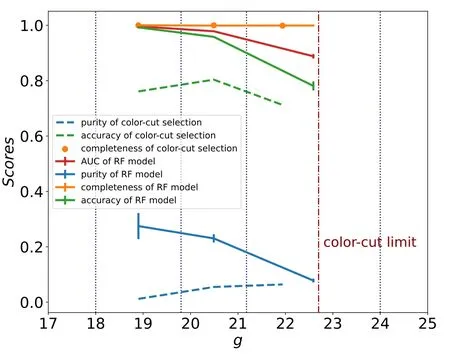
Figure 6. The results when the RF model (solid lines) and color-cut selection(dashed lines)are applied to the testing set.The testing set is divided into three subsets according to their g-band magnitudes. The details are given in Section 4.1. When testing the color-cut selection, a limit magnitude is used(detailed at Section 3.2) and shown with the red dotted–dashed line.
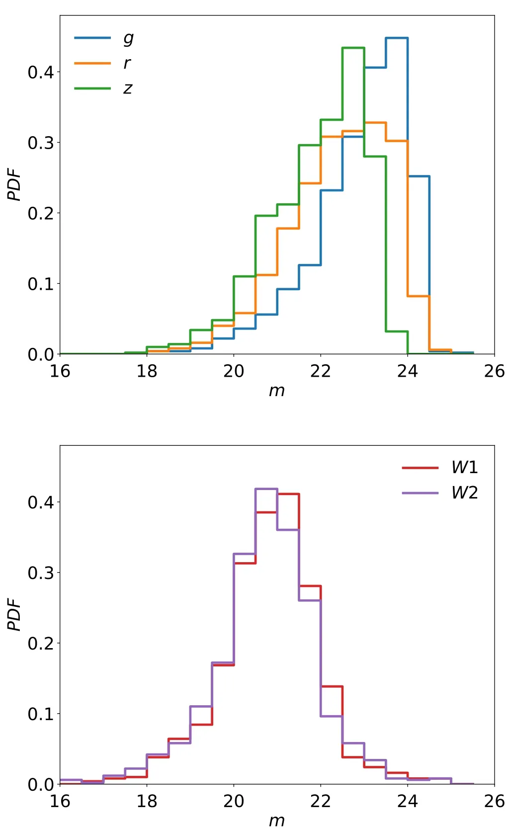
Figure 5. The distributions of g, r, z, W1, W2 of all quasar candidates.
We acquire 24,440,816 quasar candidates, and the magnitude distributions are shown in Figure 5. To evaluate the completeness, purity, accuracy, and AUC of the classification,our RF model is applied to the testing set, and the result is shown in Figure 6. The completeness remains stable while the other metrics drop significantly at the faint end.The three bins of the testing set are divided by g-band magnitudes given below, and each bin contains similar amounts of unique sources:
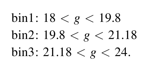
We split the sample into Grade-A and Grade-B with a g band magnitude of 21.18 because the purities of classifying the objects below and above the magnitude are significantly different. Grade-A and Grade-B contain 1,953,932 and 22,486,884 candidates separately.
The above classification is constructed by defining a threshold of the probability given by our classifier, where Pth=0.5. Correspondingly, Grade-A has the purity ~0.3 and accuracy ~0.99; Grade-B has the purity ~0.15 and accuracy~0.90. Notably, the completeness remains high in all magnitude bins(see the orange line in Figure 6).The errorbars represent the uncertainties by bootstrapping the elements in each bin (Efron 1982). Expressly, larger errorbars of purity in brighter bins are due to the fewer quasars; larger errorbars of accuracy in fainter bins are due to the decreasing capacity of the RF model.
To further investigate the effects of the thresholds of the probability of being a QSO on the performance of the classification, we test 0.5, 0.6, 0.7, 0.8, 0.9 as Pth, and the result is shown in Figure 7. In all cases, the completeness is higher than 0.85,and the completeness is even higher than 0.99(see the green filled region) when Pth={0.5, 0.6, 0.7}, but it decreases to 0.95(see the purple filled region)when Pth=0.8.Therefore, Pth=0.5 is for general purpose, and it gives high completeness but low purity. However,one can change Pthfor a specific combination of completeness and purity according to the tendency shown in Figure 7.
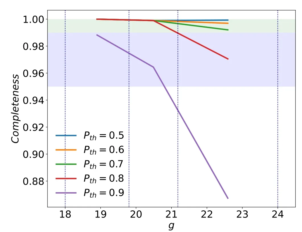
Figure 7.The variety of completeness when different Pth are applied.The way of splitting testing set is the same with the ones for Figure 6.The area where the completeness higher than 0.99 is filled by green, while the ones higher than 0.95 is filled by purple.
Considering the various setups of DECaLS and BASS+MzLS, the corresponding QSO candidates in their footprints have different statistical properties. As displayed in Figure 8,the g-band magnitudes distribution and g-z distribution are identical in DECaLS and BASS + MzLS footprints for Grade A candidates due to their higher confidence. But for Grade B candidates, the most significant difference between the magnitude distributions of the candidates in DECaLS and BASS + MzLS footprints is in the g-band because the most notable difference is in the efficiency of the g-filter of DECaLS and BASS. The Grade B candidates in DECaLS are shallower than those in BASS + MzLS in the g-band and are slightly bluer than those in BASS+MzLS when choosing g-z as the color indicator. To quantify the influences of the above differences on the identification of quasar candidates, we explore the performance of the classification when the RF models are individually trained by DECaLS (or BASS+MzLS). As shown in Figure 9, the overall performances(represented by the area under the ROC, a.k.a AUC) with the new training strategy are slightly better than the earlier one which ignores the different setups between DECaLS and BASS+MzLS.However,the differences in completeness(i.e.,TPR)are ~1‰when we choose 0.5(the adopted value in this work)as the classification threshold, while FPRs and Purity increase 10%–20% (see cross-marks and plus-marks in Figure 9, and Table 3 for explicit values).For others’convenience,we attach catalogs of quasar candidates obtained by adopting the latter training and classifying strategy as complementary to the earlier results, which can be found in the same repository.17https://github.com/EigenHermit/he-li2021
4.2. Cross-validation
To cross-check the QSO candidates found by our classifier,we identify QSO candidates using the color-cut selection independently, and the selection criteria are listed in Section 3.2. Consequently, 8,425,413 and 19,575,604 candidates are found by the RF model and color-cut selection separately. There are 6,909,375 candidates discovered using both approaches, i.e., ~82% RF candidates retrieved by the color-cut selection, as shown in Figure 10. The red line represents the hard edge of the color-cut selection, and the color-cut selection discards the RF candidates below this line.The hard-cut leads to ~18%of the RF candidates missed by the color-cut selection because the RF selection gives an irregular shape in the color space. On the other hand, 12,666,119(~65%) of color-cut candidates are new compared to RF candidates because the color-cut selection has lower purity than the RF model(see the blue dashed line in Figure 6),bringing in plenty of FP.
Furthermore,we test the Grade-A and B candidates in colorcut space as shown in Figure 11. Quantitatively, ~91%(1,771,762/1,953,932) Grade-A candidates and ~79%(5,137,613/6,471,481) Grade-B candidates and can be refound by color-cut selection. This result is consistent with the ones that could be read from Figure 6: the purity decrease at fainter region.
5. Discussion and Summary
In this work, we have built a catalog of QSO candidates by applying an approach based on RF to the data sets of DESI-LIS and WISE.To train our method,we construct a training set by cross-matching photometry data, including g,r,z from DESILIS and W1,W2 from WISE,with spectroscopically confirmed QSOs from eBOSS DR16Q for positives and the SIMBAD database for negatives. A testing set mocking the statistical properties of to-be-applied data in magnitude and color is also created and injected to evaluate the completeness, accuracy,and purity of the identification process. Finally, 24,440,816 QSO candidates are identified out of 425,540,269 point-like objects in DESI-LIS. In addition, we validate our results with those of the color-cut selection approach,and they match well.The catalog can be considered the reference for further observations of DESI and other spectrum surveys to identify new quasars. Relevant data including Grade-A and Grade-B catalogs, training and testing sets are available online.18https://github.com/EigenHermit/he-li2021Furthermore, the Grade-B candidates in DECaLS are slightly shallower and bluer than those in BASS + MzLS footprints due to the difference in the efficiency of the g-band filters in DECaLS and BASS (see Figuer 3 in Dey et al. 2019).However,the gap disappears in Grade-A candidates because of their high signal-to-noise ratios. The gaps lead to concerns about the selection of training strategies, i.e., whether the classifier should be trained with the data from the DESI-LIS footprint or only from the DECaLS (or BASS + MzLS)footprint. Our experiments present the completeness is nonsensitive to training strategies when we choose Pth=0.5 as the classification threshold (Table 3). Regardless, additional catalogs of quasar candidates obtained through the RF models trained with the latter training strategy are also published along with the primary catalogs for the others’ convenience.

Figure 8. The g and g-z distributions of Grade-A (first line)and Grade-B (second line)candidates that been observed in BASS +MzLS and DECaLS footprints.
According to the evaluations based on the testing set, the overall purity is ~0.25 while the completeness is higher than 0.99. We further define two grades for the candidates by placing a demarcation in g-band magnitudes, i.e., the Grade-A catalog contains 1,953,932 candidates that are brighter than g=21.18, while the Grade-B contains 22,486,884 candidates that are fainter than g=21.18. Besides, the accuracy, purity and AUC of the Grade-A catalog are all higher than Grade-B catalog’s,specifically,accuracy is ~0.1 higher,purity is ~0.15 higher and AUC is ~0.05 higher. However, the completeness of Grade-A is barely the same as Grade-B,which is above 0.85 under all test thresholds (0.5,0.6,0.7,0.8,0.9). The object is considered as a quasar candidate when its RF score is higher than thresholds.We select 0.5 as the identification threshold for general purposes. With this threshold, ~82% of the quasar candidates found by our method could be rediscovered by the color-cut selection method. Nevertheless, as is expected, a higher threshold leads to lower completeness but higher purity.Thus,one can tweak the threshold to satisfy the requirements of their own scientific goal.
We implement the search for QSOs over the whole field of view of DESI-LIS DR9, covering ~14,000 square degrees of the extragalactic sky visible from the northern hemisphere,more extensive than previous work.Besides,by evaluating the classification outcomes of the testing set, we find that the completeness of the QSO candidate catalogs has high completeness when selecting 0.5 as the identification threshold,which means that the confirmation process with DESI following our targets catalogs can achieve a QSO catalog with both high completeness and purity. However, considering the photometry data adopted in this work (g, r, z, W1, W2), the performance of the identification can be further improved with data in additional bands such as UV and radio. Moreover,blended objects contaminate the photometry catalog due to the PSF size of DESI-LIS; for instance, the objects considered as extended sources are excluded first in our work, which might include blended QSOs or blended QSOs and galaxies.Thus,to further increase the completeness of the targets catalog, one needs to conduct a deblending operation over the whole data sets of DESI-LIS before banning negatives,which is part of our further work.
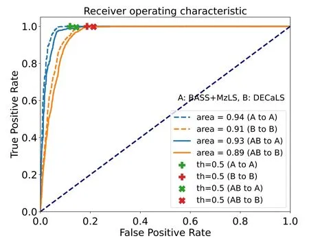
Figure 9. The ROC curves of the RF model that is trained in four different cases. The four scatters explicitly indicate the FPR and TPR when Pth=0.5.
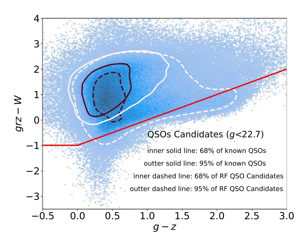
Figure 10.Two-dimensional histogram for comparing the RF model and colorcut selection.The definitions of grz and W can be found in Section 3.2 and the red-line represents color-cut condition (Section 3.2), the points below the line are discarded by color-cut selection.

Table 3 The Completeness, Purity, FPR of Four Cases when 0.5 is Adopted as Threshold
To summarize,this study provides the largest-ever catalog of QSO candidates with high completeness,which can be used for the target data set for confirming QSOs with DESI.Furthermore, grounded on this QSO candidate catalog, we are trying to find the candidates of strongly lensed QSOs with a catalog-based algorithm. So far, ~800 high-quality candidates of new strongly lensed QSO systems have been found and will be reported in a separate paper. Thorough follow-ups and analyses will be applied to the candidates. Next, we will constrain the properties of the circumgalactic medium (Cai et al. 2019; Lau et al. 2022), dark matter distribution in lens galaxies (Oguri et al. 2014; Sonnenfeld & Cautun 2021),Hubble constant(Suyu et al.2017;Liao et al.2019;Wong et al.2020) with confirmed strongly lensed QSO systems.
Acknowledgments
We thank the anonymous referee for valuable and constructive comments. We acknowledge the science research grants from the China Manned Space Project with No. CMS-CSST-2021-A01.We thank China-VO for providing DESI-LIS data and download service for our catalogs. We thank Huanyuan Shan, Rui Li,Dongxu Zhang, Heyang Liu, Jiao Li, Hao Tian, Hui Sun and Jiadong Li for the extensive discussions.We thank astropy,scikitlearn, pandas, seaborn for providing convenient and reliable python packages.
ORCID iDs
Zizhao He https://orcidorg/0000-0001-8554-9163
 Research in Astronomy and Astrophysics2022年9期
- Research in Astronomy and Astrophysics的其它文章
- A Photometric Study of Two Contact Binaries:CRTS J025408.1+265957 and CRTS J012111.1+272933
- Investigating the UV-excess in Star Clusters with N-body Simulations:Predictions for Future CSST Observations*
- A Catalog of Molecular Clumps and Cores with Infall Signatures
- Detection of 16 Small Glitches in Nine Pulsars
- Investigations of Thermal Deformation Based on the Monitoring System of Tianma 13.2m VGOS Telescope
- Simulation Study of Network Reconfiguration and Load-balancing Method for the Xinjiang Astronomical Observatory Data Center
