Two-dimensional Modeling of the Tearing-mode-governed Magnetic Reconnection in the Large-scale Current Sheet above the Two-ribbon Flare

Yining ZhangJing YeZhixing MeiYan Liand Jun Lin

1 Yunnan Observatories,Chinese Academy of Sciences,Kunming 650216,China; yj@ynao.ac.cn

2 University of Chinese Academy of Sciences,Beijing 100049,China

3 Center for Astronomical Mega-Science,Chinese Academy of Sciences,Beijing 100101,China

Abstract We attempt to model magnetic reconnection during the two-ribbon flare in a gravitationally stratified solar atmosphere with the Lundquist number of S=106 using 2D simulations.We found that the tearing mode instability leads to inhomogeneous turbulence inside the reconnecting current sheet(CS)and invokes the fast phase of reconnection.Fast reconnection brings an extra dissipation of magnetic field which enhances the reconnection rate in an apparent way.The energy spectrum in the CS shows a power law pattern and the dynamics of plasmoids govern the associated spectral index.We noticed that the energy dissipation occurs at a scale lko of 100–200 km,and the associated CS thickness ranges from 1500 to 2500 km,which follows the Taylor scale lT=lkoS1/6.The termination shock (TS) appears in the turbulent region above flare loops,which is an important contributor to heating flare loops.Substantial magnetic energy is converted into both kinetic and thermal energies via TS,and the cumulative heating rate is greater than the rate of the kinetic energy transfer.In addition,the turbulence is somehow amplified by TS,in which the amplitude is related to the local geometry of the TS.

Key words: magnetic reconnection–magnetohydrodynamics (MHD)–Sun: flares–turbulence

1.Introduction

Solar flares are the most violent events in the solar system which are involved in the conversion of magnetic energy up to 1027-1032erg.Magnetic reconnection plays a key role in this process and in helping convert the magnetic energy into heating and kinetic energy of plasma,and in accelerating charged particles.The magnetic reconnection process also widely exists in astrophysical studies including the solar atmosphere,Earth’s magnetosphere (Priest &Forbes2000),a black hole accretion disk (Yuan et al.2009;Yuan &Zhang2012;Meng et al.2015) and magnetic neutron stars(Meng et al.2014).

Several types of magnetic reconnection (MR) exist in solar activities.Parker (1957) and Sweet (1958) described a very long and thin diffusion region of an MR,which can only be used to explain slow energy releasing events.Petschek (1964)introduced a single X-type reconnection site combined with slow mode shocks in the outflow regions,in order to explain the fast MR process.Recently,turbulence has gained much attention on what kind of role it plays in the MR process.Lin et al.(2007) and Loureiro et al.(2007) pointed out that the turbulence in an MR can effectively accelerate energy dissipation in the thick current sheet (CS).Traditional theories(Petschek1964)imply that the energy is transferred from large scales to small scales and finally dissipated at the ion inertial scale,which is tens of meters in the coronal environment.However,Forbes &Malherbe (1991) and Riley et al.(2007)pointed out that the tearing mode instability plays a key role in magnetic diffusion and governs the CS thickness.Lazarian et al.(2020) suggested that turbulence requires the energy to cascade into smaller scales.The fragmented CSs and plasmoids in two-dimensional (2D) space can be classified into turbulence,while the inverse cascade of merging loops is not.How turbulence thickens CS and accelerates reconnection is quantified by Lazarian &Vishniac (1999) with theoretical predictions supported by numerical simulations (Kowal et al.2009).This means that the real thickness of the CS and diffusion scale could be much larger than the ion inertial scale.

The work by Lin et al.(2007)shows the thickness of CS can be up to 6.4×104km.Ciaravella&Raymond(2008)deduced the thickness from the Ultraviolet Coronagraph Spectrometer(UVCS) data in high temperature spectral lines [Fe XVIII] and[Ca XIV] and the value is 2.8×105km.Many observations support that the CS width reaches a quite large scale in contrary with classical theories (Savage et al.2010;Lin et al.2015;Li et al.2018;Cheng et al.2018;Yan et al.2018).In addition,numerical simulations by Mei et al.(2017) suggested the thickness can exceed 103km.On the other hand,Biskamp(1993)gave a scaling law for the Taylor scalelTthat represents the inertial-range of the energy spectrum withlT=lkoS1/6,wherelkois the Kolmogorov scale for dissipation andSis the Lundquist number,which indicates thatlTcan reach several Mm in the coronal environment.The thickness of the CS and its relation to the reconnection rate deduced by Ciaravella &Raymond(2008)could find the theoretical counterpart in Eyink et al.(2013) and Lazarian et al.(2020).However,the relation between the CS thickness and the Taylor scale length (see Biskamp1993) is not well understood.

Fragmented and turbulent CSs have been observed in detail by many works(Lin et al.2007;Savage et al.2010;Liu2013;Lin et al.2015;Li et al.2018;Cheng et al.2018;Yan et al.2018;Patel et al.2020;Lee et al.2020).Nonthermal particles observed in the solar eruption suggest the existence of turbulence,and high temperature plasma observed in some events indicates the impact of heating plasmas by turbulence(Warren et al.2018).

In the work of Bárta et al.(2011),the CS fragmentation and coalescence of plasmoids facilitate the energy release process in solar flares.Huang et al.(2017) performed a series of 2D simulations of MR in the evolving CS.They find that the classical Spitzer resistivity is important only in a narrow layer near the resonant surface inside the CS during the linear phase of the tearing mode.This layer is also known as the resistive layer (e.g.,see also Biskamp1993).The growth of the tearing mode is associated with the development of plasmoids in both size and number.As the plasmoid becomes wider than the narrow layer,the electric current density increases apparently,and oscillates violently(e.g.,see also Shen et al.2011).At this time,the initial integrity of the CS breaks down and the fast reconnection phase starts.

The 2D numerical experiments with high resolution by Dong et al.(2018) revealed that the index of the energy spectrum is about -1.5 in the inertial stage,and the copious formation of plasmoids results in a subinertial range with a spectral index of-2.2.Many dissipation sites are distributed all over the largescale CS,and the diffusion in the CS is significantly enhanced,which is equivalent to adding extra diffusivity in the reconnection region,as suggested by Lin et al.(2007) and Lin et al.(2009).In the work of Ye et al.(2019),three types of turbulence were recognized in the CS that is located between the coronal mass ejection(CME)and the associated flare.Their 2.5-dimensional(2.5D)simulation indicated that the turbulence inside the CS displays anisotropy but that on the flare loop top is roughly isotropic.

According to these works and on the basis of our previous works,we are looking into details of MR in the CS above the two ribbon flare(see Figure 1 of Kopp&Pneuman1976and/or Figure 1 of Forbes &Acton1996) via 2D simulations.To justify that we adopted a 2D model for the actual threedimensional (3D) phenomenon,we argue as follows: Unlike the reconnection process taking place in a 3D homogeneous framework (e.g.,see Kowal et al.2017,2020;Beresnyak2017),the reconnection process taking place above the tworibbon flare is highly confined to a plate-like CS,so it is an inhomogeneous process.

Both theories (Forbes &Lin2000;Lin2002) and observations (Ko et al.2003;Lin et al.2005) indicated that the solar eruption is initiated by the loss of equilibrium in the coronal magnetic configuration,and leads to thrusting the upper part of the configuration and stretching the lower part(refer to Figure 1 of Forbes &Lin2000).The disrupting magnetic configuration usually includes an electric-current carrying flux rope,which is used to model the prominence or filament that floats in the corona.Stretching the lower part of the configuration results in the formation of the CS between two magnetic fields of opposite polarity,and thrusting the upper part of the configuration (flux rope) produced an area of low pressure around the CS (see Figure 1 of Lin et al.2005).The difference in the pressure between the region near the CS and that far from the CS pushes both magnetic field and plasma to flow toward the CS,constituting the reconnection inflow(see blue arrows in Figure 1 of Lin et al.2005)and invoking the socalled driven reconnection in the plate-like CS.

Therefore,the reconnection process that we are studying here is occurring in a region that is highly squeezed in one direction by the reconnection inflow.This yields two consequences: First,MR basically takes place roughly in a 2D space;second,the process occurring in this fashion is inhomogeneous since the freedom of the process in one direction is limited.We note here that the limit to the freedom is not due to the existence of magnetic field,but due to the reconnection inflow.Hence,the reconnection process occurring in the CS above the two-ribbon flare is both driven and inhomogeneous,which is different from that studied by Kowal et al.(2017,2020) and Beresnyak (2017).This is why 2D simulations could be used for the actual 3D phenomenon of our interest.

Lazarian et al.(2020) also classified reconnection into 2D and 3D such that the tearing reconnection dominates in 2D while turbulent reconnection process plays a key role in 3D cases.Looking into details of the reconnection processes of the two kinds,we realize that the 2D process dominated by the tearing mode actually involves inhomogeneous turbulence,and that of the 3D process,which is dominated by turbulence,in fact arises from the homogeneous turbulence according to Biskamp(1993).Numerical experiments also show that the fine structures seen in planar cuts of 3D CS based on the Titov &Démoulin (1999) model are very similar to 2D simulations(Mei et al.2017;Ye et al.2019).

For the large-scale process in the early stage of reconnection occurring in the coronal environment as presented here,the frozen-in condition is only violated at places where reconnection occurs as discussed by Eyink (2015),and the scenario of the energy conversion in the CME-flare CS in the 2D fashion could still exist in reality (Guo et al.2015;Yang et al.2020;Lazarian et al.2019,2020).Hence,the reconnection process in 2D and 2.5D occurring in the CME-flare CS as a result of the tearing mode for the onset of fast reconnection is worth looking into as well.

In this work,we perform a 2D numerical study for MR in the CS occurring in the classical two-ribbon flare model(Petschek1964;Carmichael1964;Sturrock1966;Hirayama1974;Kopp &Pneuman1976;Lin et al.1995;Lin2004).In the next section,we introduce the model and the code used in this study.Section3gives the numerical results and the related analysis for reconnection,and properties of the associated turbulence.Finally,we summarize the work in Section4.

2.Numerical Models and Methods

This work focuses on the CS above the two-ribbon flare given by the CSHKP model (Kopp &Pneuman1976).Our simulation starts with a configuration in equilibrium,which includes two magnetic fields of opposite polarity perpendicular to the bottom boundary that is located on the photospheric surface.The governing MHD equations including gravity and resistivity read as:

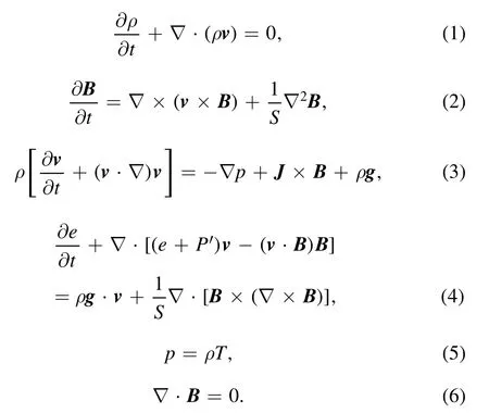
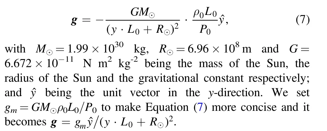
Here,all the physical quantities are dimensionless.They are almost duplicated from those of Shen et al.(2011).The quantities ρ,v,B,p,J andTare mass density,velocity,magnetic field,gas pressure,current density and temperature,respectively.The energy densitye=ρv2/2+p/(γ-1)+B2/2 while γ (set to 5/3 for the ideal gas)is the ratio of the specific heat,g is the gravity,P′ =P+B22is the total pressure including the gas pressure and the magnetic pressure,S=L0VA/η is the Lundquist number,whereL0is the characteristic length,vAis the Alfvén speed and η is the magnetic diffusivity.In our simulations,the characteristic values areB0=0.01T,L0=108m and ρ0=1.67×10-12kg m-3.Given these values,we obtainvA=6.9×105m s-1,t0=14.5 s,P0=80 Pa,J0=7.95×10-5A m-2andT0=2.90×109K as the characteristic values for velocity,time,gas pressure,current density and temperature respectively.

The dimensionless gravity reads

Regarding the initial conditions,we construct a Harris-like CS described by:

The background magnetic fieldByin our simulation implements the typical sine-type CS which follows the work by Forbes&Priest(1983),Forbes&Malherbe(1991),Shen et al.(2011),Shen et al.(2013) and Ye et al.(2020) withwin Equation(9)being the half-width of CS and set to 0.1 initially.To initiate the evolution in the system,we add a small perturbation to the initial configuration at point (0,yc) defined as

where ∊=0.03,lx=0.01,ly=0.01 andyc=0.5 are the amplitude of the perturbation,dimensionless perturbation wavelengths inx-andy-directions and the location where the perturbation occurs,respectively.

The initial temperature and pressure distributions are set as below:

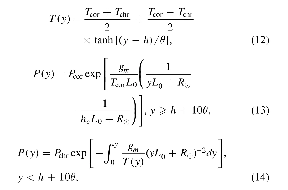
where

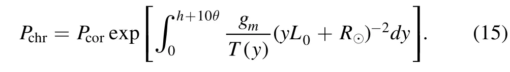
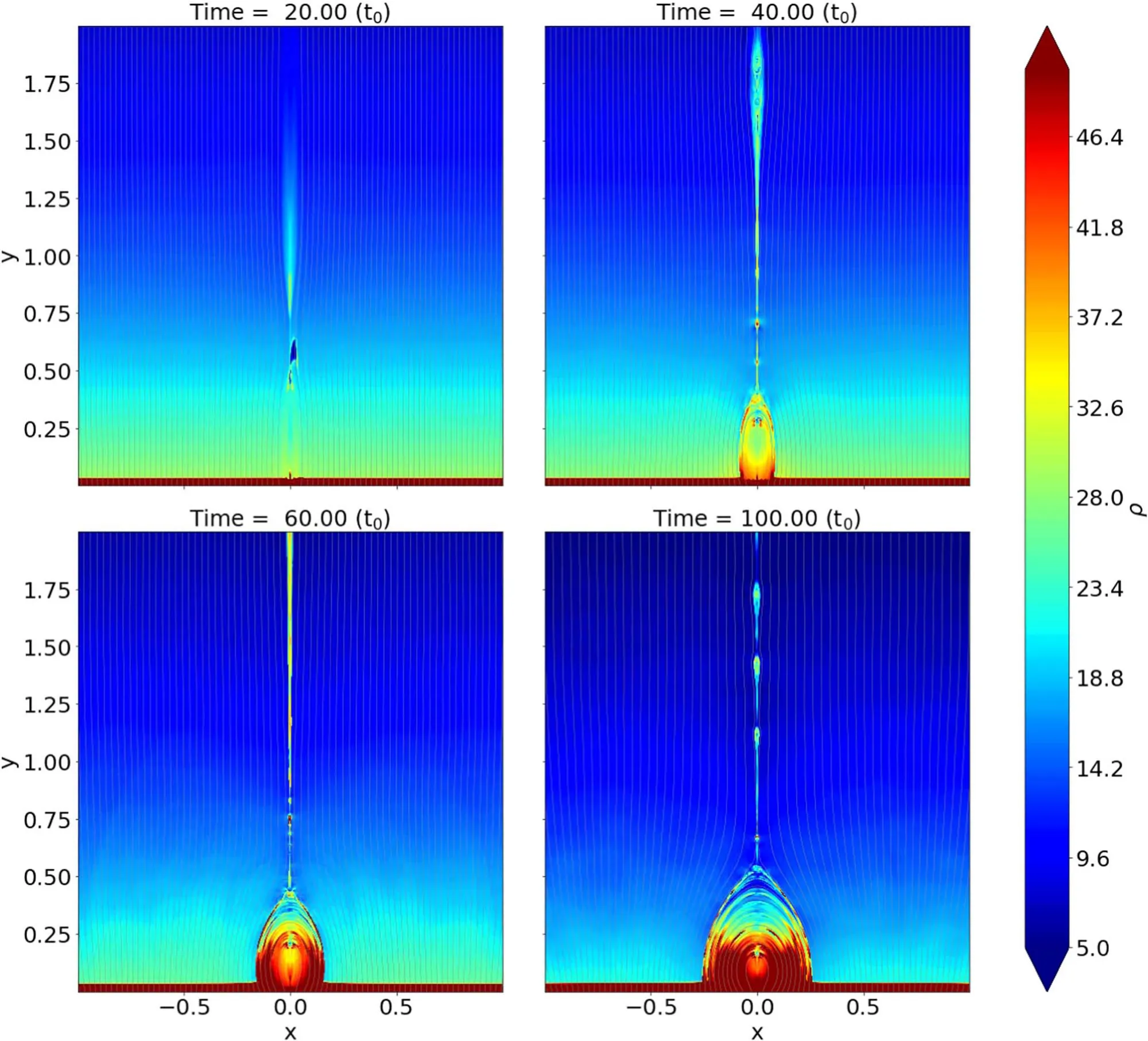
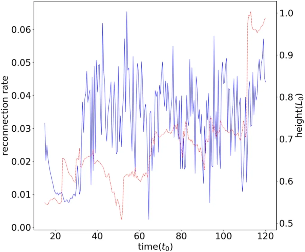
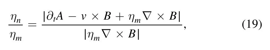
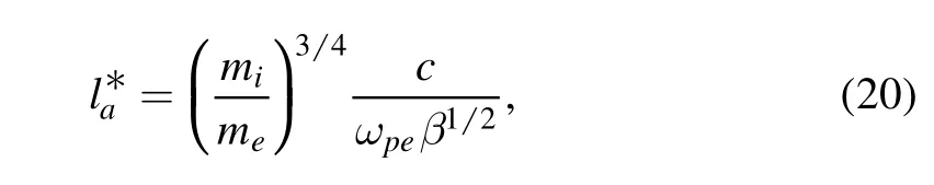
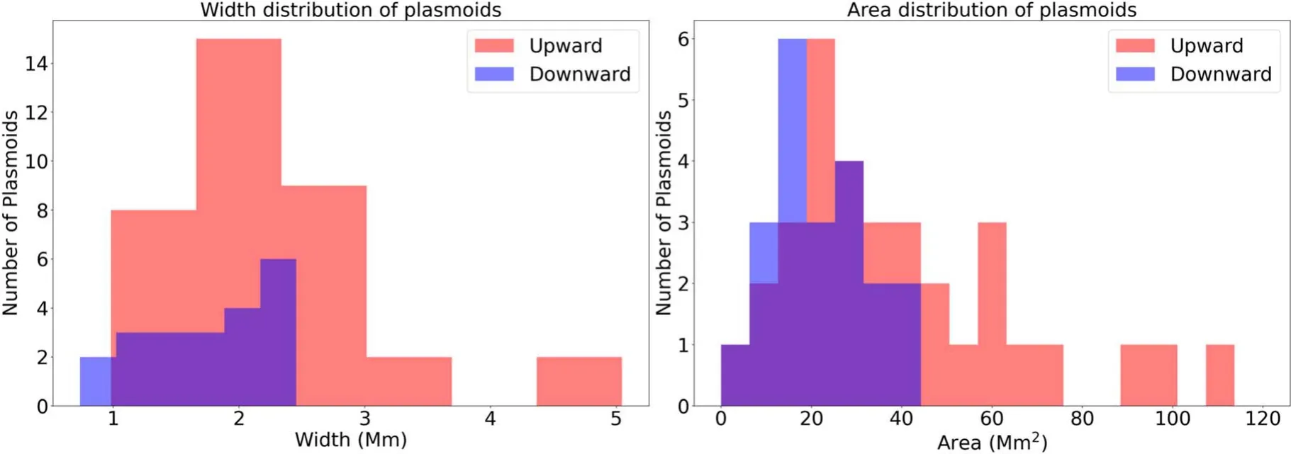
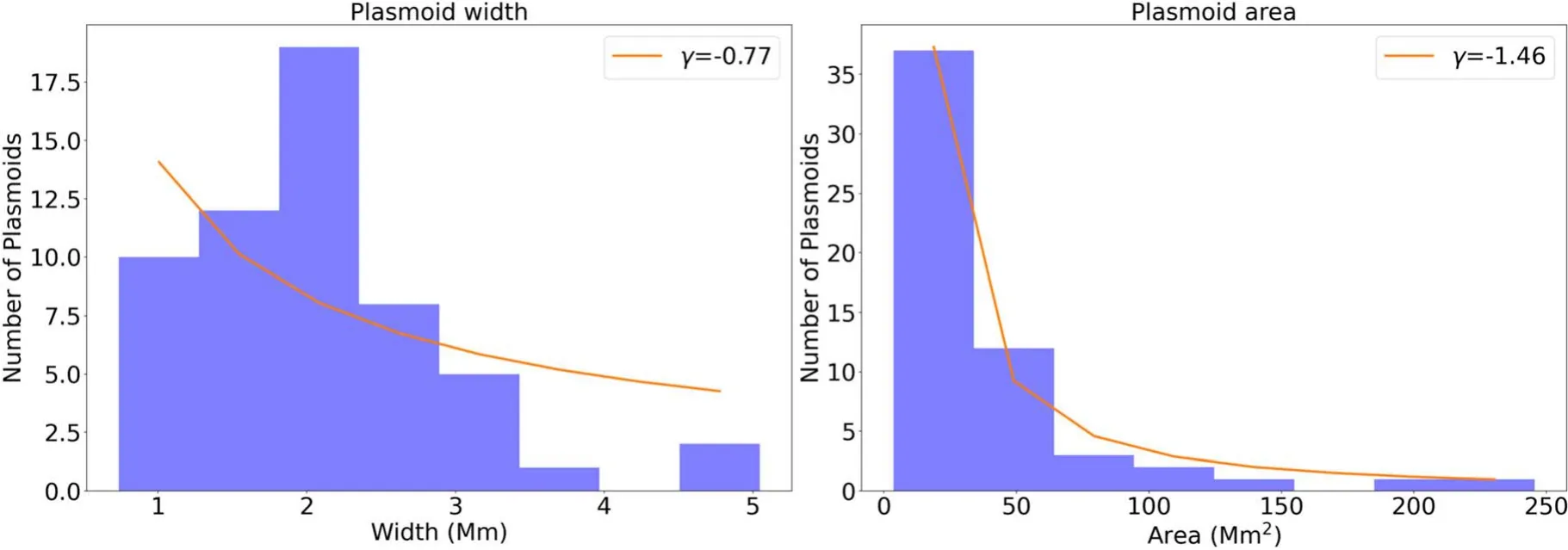
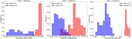
In the above equations,Tcor=6.90×10-4andTchr=1.90×10-6are the dimensionless temperatures for the corona and the chromosphere,respectively.Fory

As for boundary conditions,we set the line-tied boundary at the bottomy=0,and an open boundary for the other three sides,through which plasma can enter or exit freely.Following Shen et al.(2011),we have the magnetic field

To prevent the plasma at the bottom from slipping,we have

and for mass conservation on the bottom,we have

The simulation is performed using the ATHENA code v4.2 developed by Stone et al.(2008).We first performed our simulations under three grid resolutions of 1920×1920,3840×3840 and 7680×7680 to look into the impact of numerical diffusion on the physical scenario.The results suggest that the impact in the case of 1920×1920 is too apparent to allow the behavior of the system to match the setup of the Lundquist number,sayS=106.Ye et al.(2020)pointed out that the numerical diffusion due to the low grid resolution may suppress the effective Lundquist number.Therefore,we choose the results corresponding to the high grid resolution to perform further studies in the work below.

3.Simulation Results

3.1.Global Evolution

The global evolution in the CS is displayed in Figure1which shows mass density distribution in the time interval fromt=20 tot=100.The simulation starts with the CS being squeezed quickly near a specific point and the flare loop begins to appear at the bottom.As the CS becomes thin enough,the tearing mode instability takes place and many plasmoids are produced with multiple X-points occurring between every pair of plasmoids.In this process,that specific point eventually evolves to an X-point at which MR always happens faster than at any other X-points.This special X-point is defined as the principal X-point (PX-point).Att=40,the first plasmoid appears in the CS and the reconnection enters the impulsive phase with more plasmoids appearing and moving bidirectionally.Some of them fall and collide with flare loops and finally form a dense shell of flare loops,while the others move upwards and flow out of the upper boundary.Later att=60,a low-density cavity is formed above the flare loop.Att=100,the bidirectional moving plasmoids are clearly seen in the reconnection outflows.

Motions of the PX-point shown in Figure2display a very different feature from those in Shen et al.(2011),which indicates that the PX-point moves upward with a small amplitude oscillation around the stagnation point (S-point),and the reconnection outflow right behind the plasmoid moves faster than this plasmoid.Figure2affirms that the PX-point moves in a similar fashion at the beginning untilt=40 when it starts moving downward,and manifests a jump at aboutt=50.The same pattern repeats att=90 andt=110.Looking carefully at the reconnection process and the motion of plasmoids created in this process,we realize that gravity plays an important role in the kinematic behavior of plasmoids.

Shen et al.(2013) pointed out that a plasmoid continues to grow in both mass and volume after formation as MR progresses.In the case that gravity is absent,the motion of the plasmoid is not affected by mass accumulation;when the impact of gravity is included,on the other hand,the situation changes.With the continuous increase in mass,the impact of gravity on the plasmoid motion becomes more and more apparent.As the initial kinetic energy possessed by the upward plasmoid after leaving the PX-point is totally converted into gravitational potential energy,and the reconnection outflow behind is unable to push the plasmoid to move further upward,the plasmoid will turn to move downward.This forces the PXpoint and other plasmoids below to fall together and eventually merge with the flare loop.The previous PX-point disappears and the associated magnetic structure is destroyed as well.Meanwhile an ordinary X-point above the heavy plasmoid automatically upgrades to the new PX-point.This process happens very quickly,and almost at the same time as the previous PX-point disappears,the new PX-point is determined.Thus we see from Figure2that a jump in the PX-point height occurs following a gradual descent of the height.As for which ordinary X-point upgrades to the new PX-point,it is an open question,and we shall investigate it further in the future.

We then evaluate the reconnection rate near the PX-point in the way of:MA=vin/vAwherevinandvAare the inflow velocity and the local Alfvén velocity near the PX-point,respectively.As demonstrated by Figure2,the reconnection goes slowly at the beginning of the simulation.As the tearing mode instability is invoked in the CS,the process turns into the fast reconnection phase,and the reconnection rate jumps from 0.01 to 0.04-0.06.

Figure 1.Snapshots of the density distribution at time t=20,40,60 and 100.The gray lines describe the magnetic field at different times.

Figure 2.Reconnection rate and PX-point height in the simulation with grid resolution of Ng=7680×7680.The blue solid line represents the evolution of reconnection rate.The red dashed line shows the height of the PX point in the simulation.

3.2.Numerical Diffusion and Extra Dissipation

In our simulation,the Spitzer resistivity is set to be 10-6.Of course numerical diffusion is inevitable.The numerical diffusion enhances the dissipation in the fluid,decreases the effective Lundquist number and thus suppresses the occurrence of the tearing mode instability.Shen et al.(2011) used the AMR-improved SHASTA code with the grid size of 333 km to study the fine structure in the CS and found that the numerical diffusion introduces about a 20%error into the calculation.Mei et al.(2012) studied the eruption of a magnetic flux rope applying NIRVANA code with a grid size of 2000 km and reported that the numerical diffusion ranges from 10 to 20%of the physical diffusion.Ye et al.(2019) also used the NIRVANA code to study the energy cascading in the CS with the smallest grid size of 7.5 km.They showed that the equivalent numerical diffusivity starts from 12% at the beginning,but drastically falls to 4% and tends to be flat around 2% once AMR is turned on.They found that for the case of the Lundquist numberS=106,the resolution of 3840×3840 could apparently suppress the numerical error and allow the effective Lundquist number to match the prerequisite one.

For the physical scenario manifested by the system we are investigating,the numerical diffusion is considered extra in addition to the classical (or Spitzer) diffusion.Here using the term“extra”implies that the numerical diffusion itself is not the only issue that may impact the reconnection process,and that the so-called extra diffusion as a result of turbulence could be another issue that may govern the energy conversion in a more apparent way (e.g.,see Lin et al.2015;Ni et al.2018;Shan et al.2021).Following the practice of Shan et al.(2021),we study the extra diffusion by looking at the ratio

where ηnrepresents the extra diffusivity,ηmsignifies the Spitzer resistivity and A is the associated magnetic potential vector.We note here that the ratio in Equation(19)is evaluated in the fashion of average over a region near the PX-point in order to suppress unnecessary errors.

In addition,we note here that,in principle,the impact of the numerical diffusion on the reconnection process could be calculated via the induction equation directly.We point out that,on the other hand,since second order differentiation is involved in the calculation and more extra error could be introduced if the induction equation is directly used,we choose to evaluate the impact of numerical diffusion via Equation(19)instead.Although Equation(19)here has the same form as that of Mei et al.(2012),it possesses a different meaning here.

To evaluate this ratio,we use the “Userwork-in-loop” block in the ATHENA code(Stone et al.2008)to compute it at each timestep in simulations.This calculation can effectively improve the accuracy compared to the calculation outside the loop,and the ratio in our simulation is depicted in Figure3.

Figure 3.Ratio of extra diffusion in the simulation to ohmic diffusivity with time.The blue line shows the primitive ratio calculated in the numerical simulation,and the red line is the average ratio.

In principle,the numerical diffusion itself,for a given algorithm and the associated grid resolution,is roughly fixed.In the initial stage of the simulation,the reconnection process goes very slowly and the ratio is about 0.2-0.3 as depicted in Figure3,which is consistent with the result of Shan et al.(2021),and could be ascribed to the numerical diffusion.With the appearance of the plasmoid in the CS,the ratio increases dramatically.Consequently,a lot of plasmoids are formed,which suggests the occurrence of the tearing mode(Furth et al.1963).The ratio jumps to the range from 5–10 correspondingly.This implies that the extra diffusion becomes dominated by another dissipation term as a result of the fast reconnection phase as indicated by Eyink et al.(2011) and Lazarian et al.(2020).However,we should note here that fast reconnection accelerates the dissipation of the magnetic field,and the magnetic energy is mainly converted to kinetic energy in this process,which is basically different from the resistivity effect which transfers magnetic energy into ohmic heating (see also Eyink et al.2011;Lazarian et al.2020).

3.3.Energy Spectra Analysis

MR produces several open issues about how energy is transferred from large inertial scale to small dissipation scale.It is widely accepted that this transfer is realized by an energy cascading process as a result of turbulence.The tearing mode instability triggers the fragmentation of the large scale CS and invokes the fast energy conversion on a small scale.Our numerical simulation duplicates this process.Usually the energy spectrum for this process possesses a double power law-like pattern,which demonstrates how the energy cascades from large-scale structure to small-scale ones,and at which scale the Spitzer diffusion starts to become dominant.This process could be displayed by the distribution of the magnetic energy (Em) in the CS versus the wavenumber of the turbulence.Bárta et al.(2011) and Mallet et al.(2017)discussed the power law distribution of energy in the inertial and dissipative ranges.Bárta et al.(2011) investigated the impact of fine structures in the CS on the energy spectrum.Their 2.5D simulation indicated that the fragmented reconnection process yielded the spectral index to be about-2.14 in the scale range from 300 to 10,000 km,and the inertial stage of energy cascading ends at about 300 km.Results of Mallet et al.(2017)for the energy spectrum manifested a double power law form,and indicated that the spectral index in the inertial range is between -5/3 and -2.3.

To investigate the energy conversion process,we use fast Fourier transform(FFT)to deduce the magnetic energy spectra in the CS during the steady reconnection phase.When the tearing mode instability happens in the CS,plasmoids appear and interact with one another.When plasmoids move upward,some of them will catch up with ones ahead and merge into a bigger one eventually,and the secondary reconnection process takes place during the merging,in which many more smaller fragmented CSs are formed between two merging plasmoids,enhancing the magnetic field dissipation.

Figure4displays the evolution in the CS fromt=37.0 tot=38.5 and shows more details of the secondary small scale structures,as well as their merging.The density distribution between two merging plasmoids looks apparently chaotic and many Sweet-Parker-type CSs appear associated with multiple X-points,which suggests that the diffusion region is spread out all over the large-scale CS.A one-dimensional (1D) Fourier transform for the magnetic energy distribution along they-axis is performed,and results are expressed in Figure5.The power law or double power law distribution pattern can be seen easily,and the corresponding spectral indices are also given.

We notice that before the merging of two plasmoids att=37.0,the energy spectrum presents a single power law tendency,and the spectral index γ is about -3.01.When the two plasmoids collide and merge together att=37.5 andt=38.0,the magnetic energy spectra show a tendency of a double power law distribution.The turning points of wavenumberkis atk≃1,500 andk≃1,600 respectively.The corresponding dissipative scales are about 125 km to 133 km respectively,which are consistent with the width of the fragmented CS appearing between two merging plasmoids whose width is about 192 km.We also calculate more cases and find the width of these fragmented CSs ranges from 100 km to 200 km which is consistent with the scale associated with the turning point in the double power law spectrum.We further use the zero-padding FFT method to check the energy spectra obtained in the case of the grid resolution 3840×3840.We find that the turning point does not apparently displace.

We note here that the scale on which the dissipation becomes dominant in the turbulence is usually believed to be the inertial scale of ions,which is about 102m in the coronal environment,according to the theory of classical(namely Spitzer)resistivity.However,this scale obtained here is in the range from 100 km to 200 km as indicated in Figure5.This implies a big difference between the expectation of the classical theory and the results here.If the dissipation of the magnetic field occurs only through the Spitzer resistivity,the dissipation scale should stay at a very low level.In reality,on the other hand,the Spitzer resistivity can never be the only dissipative source.For example,the anomalous resistivity due to the ion-acoustic and lower hybrid drift turbulence could produce a dissipative process that is almost 7 orders of magnitude faster than that resulting from the Spitzer resistivity.According to Strauss(1986),the largest scale on which the anomalous resistivity starts being effective is given by

Figure 4.Evolution of density and current density at time of t=37.0, t=37.5, t=38.0 and t=38.5.Letters “x” and “o” mark the X-point and the O-point at multiple secondary MR sites respectively.

Figure 5.Magnetic energy spectra using the 1D FFT technique during a plasmoid collision process.Blue lines are the FFT energy at t=37.0,37.5 and 38.0.Red and yellow lines at each time are the fitted power law distribution of magnetic energy.The legends in the upper right show the fitted power indices.

where ωpeis the electron plasma frequency and β is the plasma β in the system of interest,which is 0.1 in this work,and c is the light speed.

According to the setup for the present simulation,the electron density near the CS is about 109cm-3,which gives ωpe=1.78×108Hz.Substituting the values of ωpeand β into Equation(20),we have= 149km.Apparently,this scale is large compared to the ion inertial scale in the corona.Strauss(1986) pointed out that in the quiet coronal environment,the hyper-resistivity is 9 orders magnitude higher than the anomalous resistivity;and Lin et al.(2007) found that,in the CME/flare CS,the difference is 4∼5 orders of magnitude.The result of Strauss (1986) also indicated that both the anomalous and hyper resistivities depend inversely on the scale of the diffusive structure quadratically.Therefore,in a turbulent CS,the scaleon which the hyper-resistivity tends to dominate diffusion should be related toand the ratio,Rha,of hyper to anomalous resistivities in the way ofwithRharanging from 104to 105.Thus,we foundranges from 149 km to 472 km,which is consistent with what we obtained earlier for the dissipative scale deduced from the turning point of the double power law spectra.

This indicates that in a turbulent reconnecting CS,the Kolmogorov microscale could be as large as a few 102km due to the occurrence of hyper-resistivity.In the spirit of Biskamp(1993),we realized thatlkocould be somehow related to the thickness,d,of the CS in which turbulent magnetic reconnection is progressing.Biskamp(1993)pointed out that an intermediate spatial scale,the Taylor microscalelT,exists between the global scale of the systemLand the dissipation scalelko.This means thatLcascades tolkosmoothly vialT,andlTis still located in the inertial range.According to Biskamp (1993),,solTis between 103km and 2×103km,andlkobetween 100 km and 200 km.

Values oflTdeduced here remind us of another important scale in the configuration of MR,namely the thickness of the CS,d.Upon examining the electric current distribution inside the CS along thex-direction obtained from our simulations,we notice that the profile of the electric current varies from place to place due to turbulence in the CS.However,the full width at half maximum of the profile is between 1.5×103km and 2.5×103km,which is consistent with both observations(e.g.,see also Savage et al.2010;Ciaravella et al.2013;Seaton et al.2017;Yan et al.2018;Cheng et al.2018;Li et al.2018)and the value oflTdeduced above.This further suggests that the turbulence occurring in the CS greatly speeds up the energy dissipation and allows it to happen at a much larger macro scale,and that the thickness of a turbulent CS should be the Taylor microscale of a few 103km in the coronal circumstance.We also estimate the value oflTdeduced from the results of Bárta et al.(2011),Shen et al.(2013),Ni et al.(2015),Ye et al.(2019) and find consistency with thelTvalue obtained in the present work.

3.4.Width and Area Distribution of Plasmoids

Copious plasmoids are generated because of the tearing mode instability in the CS and move bidirectionally(Figure1).The downward moving plasmoids eventually collide with flare loops and merge into the flare loop system,while the upward moving plasmoids successfully leave simulation domain.Shen et al.(2013) investigated the width distribution function of the plasmoids in the CS,and found a power law distribution in the way ofw-2,withwbeing the width of a plasmoid.Following Clauset et al.(2009) that gave the power law distribution via the maximum likelihood approach,on the other hand,Patel et al.(2020) deduced the distribution function of the plasmoid size asf(W)∼w-1.12.

We are able to perform a similar statistical study for our results.We selected 55 plasmoids with 36 moving upward and 19 downward.Distributions of plasmoid number versus width and area are shown in Figure6,which indicate that the width of a plasmoid could be up to 5×103km,while the area up to 108km2.We noticed that our results are consistent with those of Patel et al.(2020) who showed that the width of plasmoids can be up to 104km and the area can reach up to 8×107km2.

The average width of these plasmoids in our work is about 2.07×103km and the average area is about 4.13×107km2,while the median width is about 1.97×103km and the median area is about 2.95×107km2.Particularly,the sizes of plasmoids moving upward and downward show little difference.For downward plasmoids,the average width and area are 1.73×103km and 2.08×107km2respectively,while for upward ones they are 2.26×103km and 5.21×107km2.As for median values,the width and area for downward plasmoids are 1.72×103km and 1.66×107km2while those for upward ones are 2.09×103km and 3.19×107km2,respectively.These results are listed in Table1.Usually,both the magnetic and gas pressure are stronger at the lower altitudes than at the higher altitudes,so the upward moving plasmoids expand more easily and faster than those moving downward,which accounts for the fact that the upward moving plasmoid is fatter than the downward moving one.

Table 1Statistical Features of Plasmoids Moving Upward and Downward,as well as All Plasmoids

Furthermore,we plot numbers of all plasmoids observed moving both upward and downward against width and area of the plasmoid in Figure7,in which the left panel is for the number versus width and the right panel for the number versus area.Fitting these two distributions to the power law function yields the indices of-0.77 and-1.46,respectively,which are basically consistent with the results of Shen et al.(2013) and Patel et al.(2020).

Figure 6.Distribution of plasmoid numbers vs.plasmoid width(left)and area(right).The red histograms represent plasmoids moving upward while blue ones signify plasmoids moving downward.

3.5.Termination Shock and Energy Accumulation Rate

TS above the flare loop region is also a topic which attracts much attention in solar physics.It includes many complex structures and plays an important role in energy conversion.It forms between the top of the flare loop and the bottom of the CS.Forbes &Acton (1996) pointed out that the TS is a result of the interaction of the supersonic reconnection outflow moving downward with the closed flare loop.Figure8shows the distributions of density,Mach number and plasma β near the flare loop-top at timest=45.0,52.5 and 71.0,from left to right respectively.A significant change in the density on both sides of TS and an apparent dividing line which is the shock front can be recognized.The Mach number distribution indicates the supermagnetosonic nature of the reconnection outflow,and it ranges from 1.0 to 2.6.The Mach number of the reconnection outflow before the TS could somehow indicate the energetics of the downflow.We notice that values of the Mach number before TS at the above three moments are 2.32,2.30 and 2.42,respectively;and att=71.0,the downflow becomes more energetic,and the corresponding plasma β in the related region could reach up to unity.From the density distribution,we obtain the compression ratios across TS at the above three moments,which are 2.33,2.63 and 2.67,respectively.More values of the compression ratio at several other times are deduced as well,and the result shows that the compression ratio across the TS is between 2 and 3.

During the whole process,we notice that TSs have different geometries in various stages.Three main shapes are found,including those of linear,V-like and inverse-trapezoid types as shown in Figure8.The linear pattern of TS front,no matter if horizontal or oblique,mainly results from the interaction between the reconnection outflow and flare loops,while the V-like pattern and inverse-trapezoid pattern are generally the result of the collisions of plasmoids with the flare loop.

To look into how the shape of TS affects the turbulence strength,we use the standard deviation(STD)of velocity as an index of the turbulence strength before and behind TS.Generally,the velocity of the downward reconnecting outflow before TS is more uniform than that behind TS.Figure9displays the histogram for the frequency at which a given velocity of the plasma flow occurs either before(red)or behind(blue) the TS.We notice that the distributions of the velocity before TS are usually less dispersive than those behind TS,namely the flow velocity behind the TS spreads in a wide range with large STD.On the other hand,the mean velocities before the TS are apparently higher than those behind the TS,which suggests the occurrence of a sharp deceleration of the plasma flow across the TS.

Figure 7.Distributions of numbers of all plasmoids observed moving both upward and downward vs.width(left)and area(right).The histograms are for the numbers of plasmoids in each width/area range including both upward and downward plasmoids.The orange lines are the fitted power law distribution of the width or area.The indices of the power law distributions are -0.77 and -1.46 for width and area,respectively.

Comparison of various shapes of TSs confirms that the more asymmetric and irregular the TS,the more turbulent the region behind the TS.In particular,for the linear TS,the enhancement of the turbulence by the oblique TS is more apparent than the horizontal one.For the oblique TS that is asymmetric,the enhancement factor is between 1.5 and 2;while for the horizontal TS the factor is about 1.0.Att=45,the STD before TS is 0.0199 while that behind TS is 0.0449,leading to an enhancement factor of about 2.26.For the regular and symmetric configuration(such as that att=52.5),the STDs before and behind TS are nearly the same,say 0.02.Att=71.0 the strengthening of turbulence behind TS is quite apparent with the enhancement factor up to 2.81.Thus irregularity and asymmetry of TS structure are more efficient for enhancing turbulence.

To study the energy conversion efficiency in the region around TS,we evaluate the kinetic energy and the thermal energy.We first locate the TS position by calculating ∇·v.Due to the symmetry about they-axis,the center of TS is very close tox=0.We select Ω of [xTS(t)-0.05,xTS(t)+0.05]×[yTS(t)-0.05,yTS(t)+0.08],wherexTSandyTSare thex-andy-coordinates of TS at a given timet,respectively.The energy conversion rates for the thermal and kinetic energies are calculated in region Ω as follows

whereETLandEKLare the thermal and kinetic energies in Ω at timet,whileETIandEKIare the thermal and kinetic energies confined in Ω at timet-Δtrespectively;ETFandEKFare the thermal and kinetic energies flowing into Ω respectively;andmis the total mass in Ω and Δtis the time step for data sampling with Δt=0.1.More details about the computing approach can be found in Ni et al.(2012)and Ye et al.(2021).Our results are given in Figure10for the time interval between 20 and 80.

Figure10indicates that before the flare loop and plasmoids appear,both rates remain quite close to 0.When the CS gets thinner and thinner at aboutt=28,the tearing mode instability occurs in the CS and accelerates the energy conversion.Downward outflows collide with the closed flare loop,producing TS at the top of flare loops (Shen et al.2018).Once TS forms,both rates experience a jump and apparent energy accumulation starts.Similar processes of collisions between plasmoids and flare loops continue during the whole process and cause the successive increase in both kinetic and thermal energies.To compare the detailed accumulation of the thermal and kinetic energies fromt=20 tot=80,we integrate the rate shown in Figure10(a) over this time interval.The results are plotted in Figure10(b).We notice that before the tearing mode instability takes place,the energy accumulation is at a low level.Aftert=28,both kinetic and thermal energies experience significant increase in accumulation.Att=45,the reconnection starts the fast phase and the accumulation rates reach a plateau.

Figure10(b) also affirms that the accumulative rates for thermal and kinetic energies possess the same trend.However,the rate of increase in the thermal energy is about 4-5 times that of the kinetic one.The fact here that the thermal energy accumulates behind the TS more rapidly than the kinetic energy is consistent with the results of Murphy et al.(2011) and Ye et al.(2021).

4.Summary and Conclusions

The 3D phenomenon occurring in the two-ribbon flare was investigated via 2D simulations in this work.This could be done because of the special geometric structure of the magnetic configuration involved in the solar eruption that produced the two-ribbon flare.As Lin&Forbes(2000)pointed out,the solar eruption is associated with thrusting of the flux rope,which apparently decreases the pressure in the region where the flux rope used to stay,and severely stretches the magnetic field behind the flux rope,which develops a long CS through the low pressure region (refer to Figure 1 of Lin et al.2005).The difference in the pressure pushes both the magnetic field and the plasma toward the CS,which invokes the driven reconnection process in the CS that is obviously different from the spontaneous reconnection studied by Kowal et al.(2017,2020) and Beresnyak (2017).Furthermore,squeezing of the CS by the reconnection inflow confines all the processes occurring in the sheet to a very limited space in which the freedom in one direction is significantly suppressed.This implies that behaviors of any activities in such a sheet are inhomogeneous.Here,the inhomogeneity is not because of the existence of a magnetic field,but due to the confinement by the reconnection inflow.

Figure 8.Distributions of density and velocity (a),Mach number of the downward reconnection outflow (b) and plasma β (c) around the TS region at t=45 (left column),52.5 (middle column),and 71 (right column).The white rectangle in each panel in row (a) marks the region for evaluating the STD of velocity.

Figure 9.Histograms of the velocity distributions at t=45,52.5 and 71,from left to right respectively.Red is for the velocity before TS and blue is for that behind TS.The x-axis is for the plasmoid velocity,and the y-axis is for the normalized frequency of the occurrence of a given velocity.

Figure 10.(a)Energy conversion rates for thermal energy(left panel)and kinetic energy(right panel)with time.(b)Accumulative thermal and kinetic energy transfer rate from time t=20 to 80.The red curve is the accumulation of thermal energy while the blue one represents kinetic energy.

In this work,we focus on turbulent properties of the MR process in the CS and around the TS above the flare loop system.The Lundquist number of the system is 106,and the grid resolution for calculation is high compared to those used used in previous works (e.g.,see Shen et al.2011,2013;Ye et al.2021).Initially,MR commences in a large-scale Sweet-Parker CS.As reconnection progresses,the CS gradually gets thinner and thinner until the tearing mode instability is triggered.Plasmoids are formed inside the CS,bringing the reconnection process into the nonlinear phase.Turbulence leads to the fragmentation of the CS,and the reconnection process manifests cascading behavior.Consequently,the fast mode of MR is switched on,and complex multi-scale features appear in the CS and the region between the CS and the flare loop.We carefully studied these features and looked into their physical properties.The main results are as follows:

(1) MR continues to send plasma into the plasmoid.When getting heavy enough,an upward moving plasmoid above the PX-point may turn to fall down eventually,forcing both the PX-point and plasmoids below it to move downward together,and to merge into the flare loop system.The original PX-point structure is thus destroyed,an ordinary X-point above the heavy plasmoid upgrades to the PX-point almost instantaneously and the CS configuration including the PX-point is renewed.This phenomenon and the associated process never occurs for the case without gravity.

(2) Following the practice of previous works,we use the term“extra dissipation” to describe any effective diffusion of magnetic field in numerical experiments in addition to the Spitzer resistivity.The contribution of the numerical diffusion to the extra dissipation remains unchanged once the algorithm and the code for calculations are given.The level of extra dissipation stays low before the tearing mode.Invoking the tearing mode enhances the extra dissipation significantly within a short time.This explains why fast reconnection could still take place in a largescale CME/flare CS.

(3) The Taylor microscale of the turbulence inside the CS,lT,was found to be coincident with the CS thickness,d,which implies that the thickness of the CME/flare CS is governed by the Taylor microscale.

(4) Upward moving plasmoids are bigger than those moving downward because of the lower pressure at higher altitudes.Variations of the plasmoid number versus width and area manifest a power law feature,f(ψ)～ψ γ,with indices,γ,of -0.77 and -1.46,respectively.

(5) Three types of TSs were recognized,including horizontal,V-like and trapezoid-like styles,in the cusp region above the flare loop system.The turbulence could be strengthened by the TS.The more irregular and asymmetric the TS structure is,the stronger the enhancement is.The efficiency of energy transfer around the TS indicates that plasma heating is 5 times more efficient than acceleration,which is consistent with the result of previous works by Murphy et al.(2011) and Ye et al.(2021).

(6) Last but not least,recent work in 3D by Jiang et al.(2021) on the solar eruption indicated that the reconnection process was apparently accelerated as the plasmoid instability occurs,and turbulent features in the reconnection region were found to be similar to what has been shown in the present work.In the future,we shall perform full 3D experiments for reconnection in the two-ribbon flare CS.

Acknowledgments

We are very grateful for the referee’s valuable comments and suggestions that helped improve this article greatly.This work was supported by the Strategic Priority Research Programme of Chinese Academy of Sciences(CAS)with grants XDA17040507 and QYZDJ-SSWSLH012,the National Natural Science Foundation of China(NSFC,Grant Nos.12073073,11933009 11973083 and U2031141),grants associated with the Yunling Scholar Project of Yunnan Province and the Yunnan Province Scientist Workshop of Solar Physics,and grants 202101AT070018 and 2019FB005 associated with the Applied Basic Research of Yunnan Province.Calculations in this work were performed on the cluster in the Computational Solar Physics Laboratory of Yunnan Observatories.

ORCID iDs