Super-resolution of Solar Magnetograms Using Deep Learning

Fengping DouLong XuZhixiang RenDong Zhaoand Xinze Zhang

1 State Key Laboratory of Space Weather,National Space Science Center,Chinese Academy of Sciences,Beijing 100190,China; lxu@nao.cas.cn

2 University of Chinese Academy of Sciences,Beijing 100049,China

3 Peng Cheng National Laboratory,Shenzhen 518000,China

4 State Key Laboratory of Virtual Reality Technology and Systems,School of Computer Science and Engineering,Beihang University,Beijing 100191,China

Abstract Currently,data-driven models of solar activity forecast are investigated extensively by using machine learning.For model training,it is highly demanded to establish a large database which may contain observations coming from different instruments with different spatio-temporal resolutions.In this paper,we employ deep learning models for super-resolution (SR) of magnetogram of Michelson Doppler Imager (MDI) in order to achieve the same spatial resolution of Helioseismic and Magnetic Imager(HMI).First,a generative adversarial network(GAN)is designed to transfer characteristics of MDI onto downscaled HMI,getting low-resolution HMI magnetogram in the same domain as MDI.Then,with the paired low-resolution and high-resolution HMI magnetograms,another GAN is trained in a supervised learning way,which consists of two streams,one is for generating high-fidelity image content,the other is explicitly optimized for generating elaborate image gradients.Thus,these two streams work together to guarantee both high-fidelity and photorealistic super-resolved images.Experimental results demonstrate that the proposed method can generate super-resolved magnetograms with perceptual-pleasant visual quality.Meanwhile,the best PSNR,LPIPS,RMSE,comparable SSIM and CC are obtained by the proposed method.The source code and data set can be accessed via https://github.com/filterbank/SPSR.

Key words: techniques: image processing–Sun: magnetic fields–Sun: atmosphere

1.Introduction

Nowadays,more and more advanced solar Magnetographs are being developed to measure magnetic field strength and polarity of the Sun,for studying the source and evolution of solar magnetic field.However,different magnetographs have different resolutions,noises,saturation levels and other specifics.For example,the Helioseismic and Magnetic Imager(HMI;Scherrer et al.2012;Schou et al.2012) was operated since 2010 onboard the Solar Dynamics Observatory (SDO;Pesnell et al.2012).It can provide solar magnetogram of 05 per pixel resolution,magnetic intensity and vector magnetic field.The Michelson Doppler Imager (MDI;Scherrer et al.1995;Domingo et al.1995) was operated from 1995 to 2011 onboard the Solar and Heliospheric Observatory (SOHO),providing solar magnetogram of 2″per pixel resolution.These two magnetographs have different spatial resolutions,which impedes the joint application of them in the same forecasting task.Super-resolving the MDI magnetogram into the resolution of HMI magnetogram,we can obtain a solar flare database containing magnetograms for more than two decades,benefiting solar flare forecasting greatly.

The region with stronger magnetic field than its surrounding region in the Sun is named active region(AR).The AR is the main source of of energetic phenomena (e.g.,solar flare and coronal mass ejection (CME)).High-resolution of AR is crucial for probing mechanism behind violent solar bursts which are of great interest to scientists.In addition,uniform resolution magnetogram across different telescopes is very beneficial to statistical modeling of solar activity forecasting.Thus,super-resolution (SR) of AR/magnetogram is of great significance in both solar physics and solar activity forecasting.Recently,deep learning-based SR has been investigated in solar astronomy (Xu et al.2019;Xu et al.2020;Yu et al.2022).Anna Jungbluth et al.(Jungbluth et al.2019)leveraged HighRes-Net (Deudon et al.2019) to super-resolve the MDI magnetograms to the same resolution of HMI magnetograms.Sumiaya Rahman&Yong-Jae Moon(Rahman et al.2020)applied two deep learning-based networks to enhance the HMI magnetograms by a factor of four,and compared the generated HMI magnetograms with the Hinode/Solar Optical Telescope Narrowband Filtergrams (NFI) magnetogram.However,Jungbluth et al.(2019) is about SR of full-disk magnetogram.In addition,it uses overlapped magnetograms between MDI and HMI from 2010 to 2011.This time interval has only few ARs,resulting in low efficiency of SR of ARs.Rahman et al.(2020)only super-resolves the bicubic-downsampled HMI magnetograms,not concerning real-world scenarios.

SR reconstructs high-resolution (HR) image from lowresolution (LR) image (Freeman &Pasztor1999).Deep learning-based SR has achieved promising performance of both quantitative and qualitative (Kim et al.2016;Lim et al.2017;Zhang et al.2018b;Muqeet et al.2019).Most state-of-the-art SR models impose bicubic downsampling on HR images to get LR images paired with HR images.However,bicubic downsampling may alter image characteristics,leading to a serious problem that the downsampled LR image has distinct image characteristics different from that of real-world image,namely domain difference,including sensor noises,blur and other specifics (Lugmayr et al.2019).This would lead to the performance drop drastically when the trained model is applied to real-world scenarios.Therefore,to overcome the mentioned problem,SR methods recently applied an unsupervised generative adversarial network (GAN) model to first conduct domain migration.Manuel Fritsche et al.(Fritsche et al.2019)proposed DSGAN to introduce natural image characteristics into bicubic-downsampled images.The unsupervised DSGAN can be trained on HR images,thereby generating LR images with the same characteristics as the natural LR images.Then,the paired LR and HR images constitute a database for training SR model by supervised learning.Recently,GAN based SR network has been verified to recover photorealistic images with high-fidelity as the target images (Ledig et al.2016;Sajjadi et al.2017;Wang et al.2018;Soh et al.2019).Cheng Ma et al.(Ma et al.2020) proposed a structure-preserving SPSR model to generate perceptual-pleasant details,which leverages gradient information as the gradient branch to improve the details of SR results.

General images,in contrast to magnetograms,usually have clear semantic information and rich texture structure.Therefore,super-resolution of general image mainly concerns recovering semantic information,such as edge,structure and texture,which is closed related to perceptual visual quality.Moreover,because the structure of general images is more complex,the network of SR for general image is more complicated.In contrast,super-resolution of magnetogram is more concerned with the fidelity,the invariance of the physical parameters of the magnetic field (e.g.,magnetic flux remains constant).

The SOHO/MDI(2″)and the SDO/HMI(05)are different in noise characteristics,saturation,spectral inversion techniques and other physical characteristics,resulting in two different domains of magnetograms.To address domain difference problem,we first leverage DSGAN (Fritsche et al.2019) to perform domain migration,where the input is an HR HMI magnetogram,the output is an LR HMI magnetogram in the same domain as the MDI magnetogram.Then,a twochannel/branch GAN model,namely structure-preserving super resolution (SPSR) (Ma et al.2020) is performed to super-resolve MDI magnetogram.The SPSR takes into account gradient preservation and enhancement,which benefits to recovering the gradient of magnetogram.The gradient of magnetogram is a direct measure of magnetic gradient field on the surface of the Sun.Therefore,maintaining and enhancing the gradient is essential for generating magnetograms with both pleasant visual quality and high fidelity.

In brief,there are two key points in the proposed method for SR of magnetogram.On the one hand,the DSGAN method is first employed to accomplish domain transferring/transformation.It alters image characteristics of LR magnetogram directly downscaled from HR HMI magnetogram,converting it to the one in the same domain as MDI magnetogram.Thus,a database consisting of LR&HR magnetogram pairs can be prepared for the following supervised learning of SR model.On the other hand,the SPSR Ma et al.(2020) is employed to leverage image gradient through an additional network branch to generate pleasant structures of magnetogram.In natural image,gradients coincide with sharp edges of local image objects.Moreover,gradients of a magnetogram are direct measures of the magnetic field gradients on the surface of the Sun.However,Jungbluth et al.(2019) only leverages gradient loss in the HighRes-Net,which makes the results generally suffer from geometric distortions.Hence,we adopt SPSR method with both gradient loss and separate gradient branch to generate perceptual-pleasant magnetograms.

2.Data

SDO/HMI started observation from 2010,recording photospheric vector magnetic field at 05 spatial resolution for every 45 s,obtaining magnetograms of size 4096×4096.SOHO/MDI was operated from 1995 to 2011 with spatial resolution of 2″ and temporal resolution of 96 minutes,obtaining magnetograms of size 1024×1024.In this paper,we super-resolve magnetograms of active region rather than full-disk magnetograms.We downloaded the HMI magnetograms of active region from JSOC and imaged them.The MDI magnetograms of active region are extracted from full-disk MDI magnetograms given coordinates of active regions.MDI and HMI are two different devices,not only differ in resolution.Thus,there exists domain difference between MDI magnetogram and HMI magnetogram.To mitigate domain difference,a DSGAN model is trained to fulfill domain transfer,generating LR HMI magnetogram complying with the domain of MDI magnetogram.Using the well-trained DSGAN,we collected 70,064 LR and HR HMI magnetogram patch pairs from 2010 May to 2014 May to construct a training data set for training the SPSR model.The validation set contains magnetogram patches from May 2014 to 2014 November.The HMI magnetograms from 2014 November to 2017 April and the MDI magnetograms from 1996 July to 2010 December constitute the testing data set.It should be pointed that the magnetogram patches of the same size are used for model training,while magnetograms of any size can be the inputs of SPSR model for inference.The details of training,validation and testing data sets are provided in Table1.

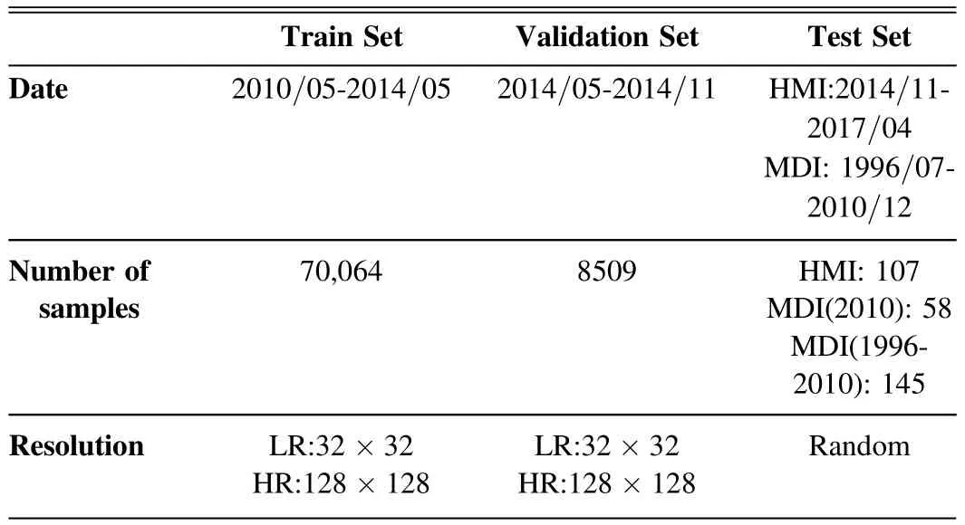
Table 1The Details of the Datasets for the SPSR Model

Table 2Comparisons of Models on Test HMI Dataset with PSNR,SSIM,LPIPS,CC and RMSE

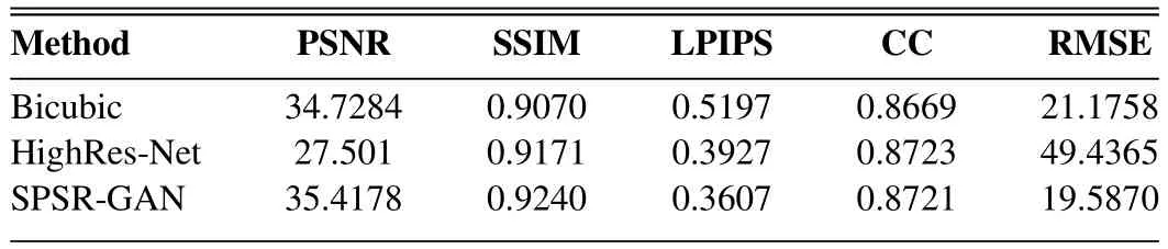
Table 3Comparisons on MDI Dataset(2010)with Respect to PSNR,SSIM,LPIPS,CC and RMSE

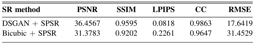
Table 4Quantitative Comparisons on the Dataset of HMI Magnetograms with Respective to PSNR,SSIM,LPIPS,CC and RMSE

3.Method

As mentioned above,the overall framework of our method consists of two stages.In the first stage,the DSGAN model is employed to accomplish domain transferring,converting directly bicubic-downscaled HMI magnetograms to the ones in the same domain as MDI magnetogram.Then,a database consisting of paired LR&HR magnetograms in the same domain can be provided for the second stage of supervised learning.In the second stage,a supervised SR model,namely SPSR,is trained over the established database in the first stage.Usually,SR may generate super-resolved images with undesired geometric distortions or twisted structure.To alleviate this problem,the SPSR is investigated for magnetogram SR in this paper.It exploits gradient as the prior knowledge.Gradient is the direct measure of magnetic gradient field on the surface of the Sun.The SPSR model can improve the subjective visual performance with rich small-scale structures and sharp edges.We describe these two stages in detail as follows.

3.1.Unsupervised DSGAN Model

In this part,we describe the overall structure of the DSGAN as shown in Figure1,where the DSGAN is exploited to generate LR images in the domainZ,given the corresponding HR images in the domainY.First,we downscale the HR images using the bicubic downsampling method to obtain the LR images y↓b=B(y).y↓bis in the domainY↓instead of the expected domainZ.To transfer y↓bto the domainZ,a generatoris applied to y↓b,to learn a mapping fromY↓domain todomain,namely=G(y↓b) .To train,a standard GAN(Goodfellow2016) with an additional discriminatorDis employed.The discriminatorDis used to distinguish the output and the source images.The output imageG(B(Y)) is regarded as the fake sample,while the source image in the domainZis regarded as the real sample.

Figure 1.Architecture of the unsupervised DSGAN model.

Figure 2.Architectures of the supervised SPSR model.

Network Architecture:The generator network contains several residual blocks (He et al.2015) with a short skip connection.Each block includes two convolutional layers with strides of 1 and a RELU activation function in between.We use 3×3 filters in all convolutional layers.As the downsampled image low frequency information remains and the high frequency information loses,we apply discriminatorDonly on the high frequency.The discriminator contains four convolutional layers with 5×5 kernels.Between each layer we apply LeakyReLU activations.The number of feature maps is increasing layer by layer,where the input channel is 3,then increases to 64,128,256.Finally,the output LR images of the generator and the source LR images are fed into the discriminator.

Loss Function: To train the DSGAN model accurately,we utilize multiple loss functions with content lossLcontent,perceptual lossLperand adversarial lossLadv.As the content attach importance to the low frequencies,we define a Gaussian low-pass filter aswL.To keep the low frequencies constant,we apply anL1loss to be the content loss,as expressed by Equation (1):

wherenrepresents the batch size.

Perceptual loss has been proposed in Johnson et al.(2016),which is effective in image restoration.It contains semantic information in the features.We apply the pre-trained VGG16 network to extract the features.It can be defined as follows:

where φirepresents the output features of theith layer.The bicubic downsampling method can only preserve low frequencies of an image,resulting in the loss of high frequencies of an image.Therefore,we apply the GAN loss (i.e.,lgenandldisk)only to the high frequencies,wherewHrepresents a Gaussian high-pass filter.The discriminator contributes to distinguishing the LR image y↓band the source LR image on high frequency.The GAN loss makes the generated LR image in the domain ˆzclose to the source image in the domainZ.The GAN loss is given as:

where λt1and λt2represent the weights of pixel loss and perceptual loss,respectively.λt3and λt4are the weights of the adversarial loss.

3.2.Supervised SPSR Model

After domain transformation,the output LR images with the corresponding HR images constitute the image pairs.The supervised SPSR model is then trained over the prepared LRHR image pairs.The SPSR model with gradient guidance preserves finer structure and high fidelity of the images.Because the gradient map reveals the sharpness and finer textures of an image,we use it to guide the super-resolution of the images.A gradient branch is used to generate the high resolution gradient maps from the LR images,providing gradient information to the SR branch.

Network Architecture: An overview of the SPSR model is depicted in Figure2.The network consists of the SR branch and the gradient branch.The SR branch is divided into four modules: shallow feature extraction,high-frequency feature extraction utilizing Residual in Residual Dense Block(RRDB)proposed in the ESRGAN (Wang et al.2019),fusion module and reconstruction module.The shallow feature module includes one convolution layer with a 3×3 filter with feature maps of size 64.The high-frequency feature extraction module contains 23 RRDB blocks and one long skip connection.The fusion model contains one fusion block which fuses the feature maps from the two branches together.Finally,the SR image is reconstructed through the reconstruction module,which has one RRDB block and a convolutional layer.The gradient branch consists of multiple gradient blocks which are employed to extract higher-level features.In addition,the gradient branch incorporates the middle-level features from the SR branch,which benefits to recovering the gradient maps.Finally,the SR branch integrates the generated SR gradient maps by the gradient branch to guide SR reconstruction in turn.

Figure 3.Visual comparison among LR,HR,our SPSR model,HighRes-Net and bicubic method on HMI images.From top to bottom,the first,third and fifth rows are full-images,and the others are zoomed-in patches.

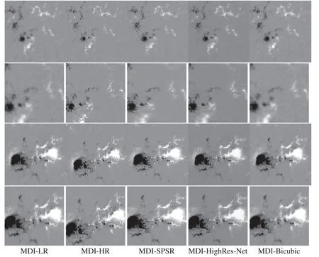
Figure 4.Visual comparison among LR,HR,our SPSR model,HighRes-Net and bicubic method on 2010 MDI images.From top to bottom,the first and third rows are full-images,and the others are zoomed-in patches.

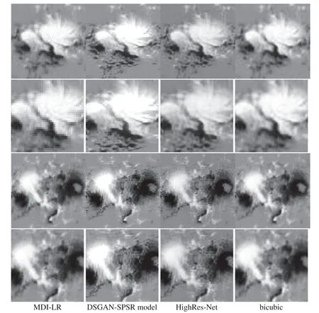
Figure 5.Visual comparison among LR,our SPSR model,HighRes-Net and bicubic method on the MDI magnetograms.From top to bottom,the first and third rows are full-images,and the others are zoomed-in patches.

Figure 6.Visual comparison among LR-bicubic,LR-DSGAN,HR,our DSGAN-SPSR model and Bicubic-SPSR on HMI images,From top to bottom,the first row is full-images,and the second is zoomed-in patches.

Loss Function:We utilize multiple loss functions containing common pixel-wise loss,perceptual loss,adversarial loss and gradient loss to train the model.The gradient loss consists of gradient pixel-wise loss and gradient adversarial loss.Both of them are applied to the gradient map of the generated SR image and HR image.The gradient pixel-wise loss and the gradient adversarial loss are given by:

4.Results and Discussion

4.1.Implementation Details

Model training details: We downsample HR HMI magnetograms by the DSGAN method to get LR HMI inputs and only consider the scaling factor of 4 in the SPSR model.First,we utilize DSGAN to generate the LR HMI magnetograms in the similar domain to the MDI magnetograms.For training the DSGAN network,we crop 128×128 HR HMI magnetograms patches and 32×32 LR MDI magnetograms patches;the batch size is 16.We train the DSGAN network with 400 epochs and use the Adam (Kingma &Ba2014) optimizer with β=0.5.The initial learning rate is 2×10−4for the generator and discriminator and decayed with the epochs.

Second,the generated LR-HR HMI magnetogram pairs are used to train the SPSR model.We randomly crop patches of size 32×32 and patches of size 128×128 from LR HMI magnetograms and the corresponding HR magnetograms,respectively.In addition,we train the model for 200 epochs and use the Adam optimizer with β1=0.9 and β2=0.999.The learning rate is set to 1×10−4,and it decayed to half by every 1000 iterations.We optimize the model using pixel loss,perceptual loss,GAN loss and gradient loss.Because the structure of the magnetograms is not complicated,the weights of the gradient loss and other image-space loss are different for the trade-off.All the experiments are implemented by using PyTorch 1.6.0.

Evaluation metrics: For quantitative evaluation,we employ PSNR,Structure Similarity (SSIM) (Wang et al.2004),Learned Perceptual Image Patch Similarity (LPIPS) (Zhang et al.2018a),correlation coefficient(CC)and root mean square error (RMSE) to evaluate our method.PSNR represents the error between the corresponding pixel points,reflecting the fidelity of the generated images.SSIM measures the imagesimilarity in terms of brightness,contrast and structure.However,the two measures do not take into account the visual recognition and perception characteristics of the human,which makes the two measures are poorly related to the human subjective perception.Therefore,we consider the LPIPS as the primary metric for comparison.LPIPS has the best correlation with both image similarity and human perception.In addition,the physics-based CC and RMSE metrics are computed over the total signed magnetic flux to evaluate the super-resolved solar magnetograms.RMSE measures the deviation between the generated magnetic flux and the observed magnetic flux.RMSE is more sensitive to the outliers.The CC reflects the degree of linear correlation between the generated magnetic flux and the observed magnetic flux.Namely,the CC and RMSE reflect the trend and the true value consistency,respectively.The RMSE and CC metric are calculated by:

whereN,are the total number of testing data,the observed magnetic flux,the generated magnetic flux,the average observed magnetic flux and the average generated magnetic flux,respectively.

4.2.The Comparison of Super-solved Results on HMI

Quantitative Comparison: In this section,we evaluate our model on the synthetic LR HMI magnetograms.We compare our model with other two methods including bicubic interpolation and a deep learning model named HighRes-Net.The HighRes-Net has been applied on solar magnetograms superresolution.In the quantitative evaluation,the results of PSNR,SSIM,LPIPS,CC and RMSE are presented in Table2.From Table2,we see that our SPSR model obtains the best PSNR,LPIPS,RMSE,comparable SSIM and CC.Our method surpasses other two methods by a large margin in terms of LPIPS benefiting from the gradient-space guidance for preserving geometric structures.Although HighRes-Net obtains the best SSIM values,it obtained the worst RMSE and PSNR values.This is due to the large deviation of the generated magnetic flux from the observed magnetic flux in the strong magnetic fields.The bicubic method obtains the second best PSNR values,it is more like a PSNR-oriented interpolation method generating blurred images.In addition,the CC value is almost equal to the HighRes-Net method,while the RMSE values surpass HighRes-Net by a large margin,indicating that our method has good stability while generating magnetic flux values are closer to the observed magnetic flux value.

Qualitative Comparison:We show a visual comparison of our SPSR model,HighRes-Net and bicubic method.From Figure3,we observe that our method produces perceptualpleasant results which are more realistic and natural.For the first magnetogram observed on 2015 January 3,our SPSR method can recover small-scale magnetic structures with fewer artifacts.Moreover,SPSR model can produce clear polarity inversion line and sharper edges.The bicubic method and HighRes-Net produce blurry magnetograms.Then,we apply these methods on MDI magnetograms,the results of which are shown in Figures4and5.

4.3.The Comparison of Super-solved Results on Real MDI

In this section,we evaluate our model on the LR MDI magnetograms in real scenarios.MDI and HMI observations overlapped from 2010 to 2011.However,there exists a slight time difference of image capture time,resulting in small deviation of magnetogram between MDI and HMI.We present the quantitative and qualitative comparisons of SR results over paired data of MDI and HMI in 2010.The quantitative comparison is listed in Table3.We can observe that our method achieves the best performance over MDI data set in terms of almost all the metrics.The correlation coefficient(CC)and root mean square error(RMSE)metrics are calculated from total signed magnetic flux.The quantitative comparison shows that our method is effective to the real MDI magnetogram.The qualitative experimental results are presented in Figure4,where the magnetograms were observed on 2010 May 1 and 2010 November 16.From Figure4,our method can produce small-scale structures of magnetic field,with sharper edges than HighRes-Net and Bicubic methods,which is more close to the target magnetogram in both positive and negative magnetic regions.However,the results of the HighRes-Net and Bicubic methods are much more blurred than the SPSR method.All three methods produce a better distribution of magnetic flux.

Table 5Comparison of SPSR Model with/without Gradient Guidance

Figure5presents a comparison on MDI observed on 2003 October 31 and 2000 June 7 of our SPSR method,HighRes-Net and bicubic.Since the two MDI magnetograms have no ground truth,we only show the visual quality.For the image in Figure5,our SPSR model has generated relatively clear magnetograms with detailed information and preserves finer geometric structures.In contrast,the HighRes-Net and the bicubic method produce blurred magnetograms including unnatural artifacts.The structures in SPSR method are clear without severe distortions,while other methods fail to show a satisfactory appearance for the objects.

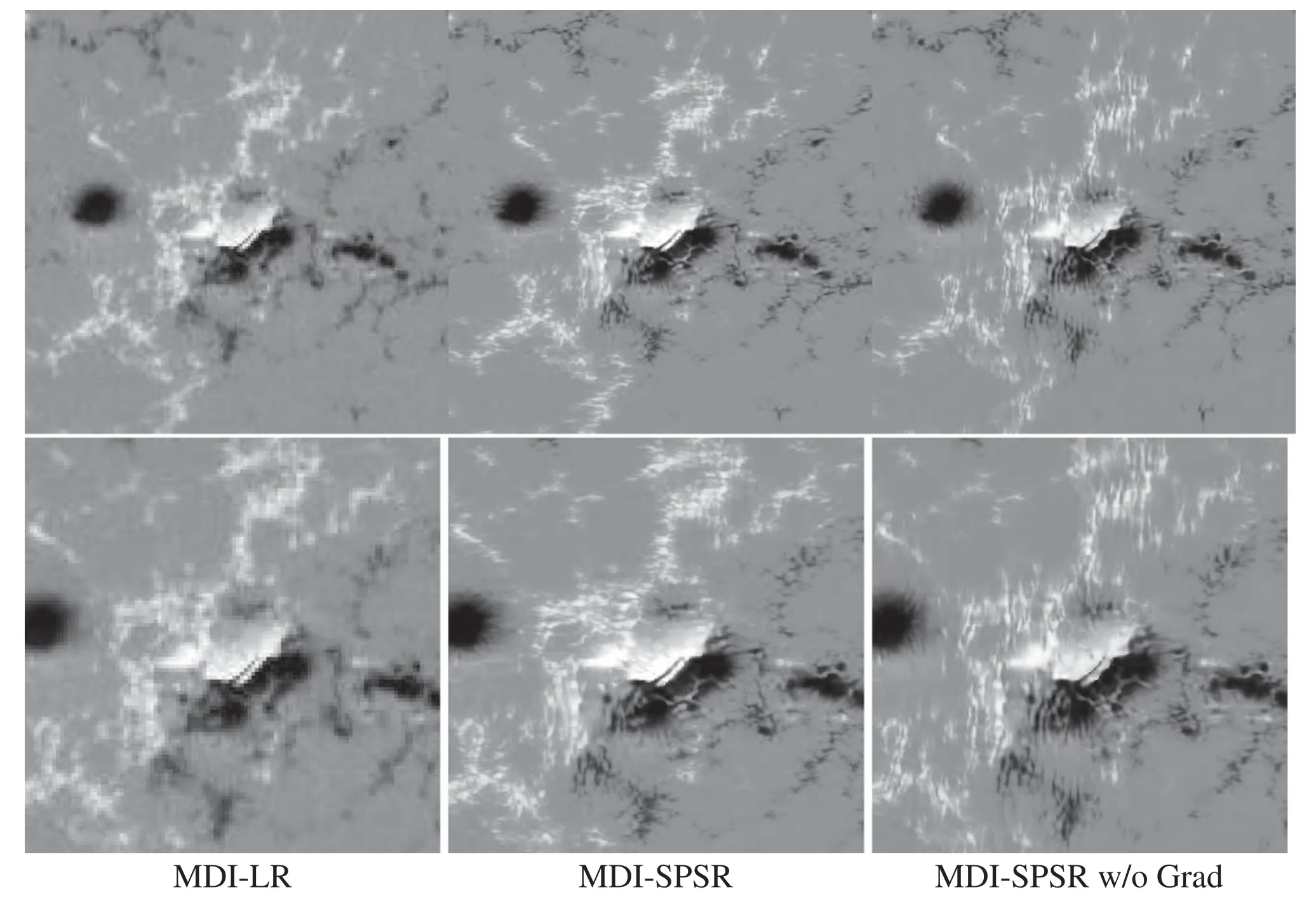
Figure 9.Visual comparison among LR,HR,complete SPSR model and SPSR model without gradient guidance on MDI images.From top to bottom,the first is fullimages,and the second is zoomed-in patches.

4.4.Ablation Study

In this section,we conduct two experiments to validate the necessity of the different downsample methods and the gradient guidance.First,we compare our DSGAN model and the bicubic downsample method.We obtain two data sets containing LR-HR HMI magnetogram pairs by the two methods.We feed the two data sets to train the SPSR model separately.Our quantitative results are provided in Table4reporting PSNR,SSIM,LPIPS,CC and RMSE.It is observed that the performance of the DSGAN method is much better than the bicubic method in all metrics,which demonstrates the effectiveness of the domain transformation.We provide visual results in Figures6and7testing on DSGN-LR HMI and MDI magnetograms.In Figure6,we see that the bicubic-LR HMI magnetogram and DSGAN-LR HMI magnetogram exit some differences.For example,the bicubic-LR HMI magnetogram is clean in the clean domain resulting from it alters the characteristics of the HR HMI magnetograms.The DSGAN model enables the generated LR HMI magnetograms in the similar domain with the MDI magnetograms.The bicubic downsampling method produces blurred magnetograms with many artifacts and incorrect structure in Figures6and7.The result indicates that bicubic method is not applicable to super-resolution of the MDI magnetograms.In contrast,our DSGAN model greatly enhanced the performance.In Figure6,the generated SR HMI magnetogram is consistent with the HR HMI magnetrograms with sharper edges and finer geometric features.In Figure7,the generated MDI magnetogram has clear edges and small-scale magnetic structures.Therefore,our DSGAN is more applicable to the super-resolution of the MDI magnetograms.

We conduct the second experiment to validate the effectiveness of the gradient loss and gradient branch.We compare the SPSR without the gradient loss and gradient branch with the complete SPSR model.Quantitative comparison is presented in Table5.We see that our complete SPSR model gets the best metrics,which demonstrates that gradient guidance can improve the model performance.The qualitative results presented in Figure8.The complete SPSR model recovers the HMI magnetogram with sharper edges and pleasant structure.However,the SPSR model without the gradient guidance recovers a blurred HMI magnetogram with incorrect structure.Figure9shows the visual results on the LR MDI magnetogram.Our complete SPSR model can recover photorealistic magenetograms without many distortions.The SPSR model without gradient guidance fails to reconstruct MDI magnetograms with clearly serrated structure.This illustrates the important role of gradient guidance for super-resolving the magnetograms with correct structure.

5.Conclusions

In this paper,a super-resolution model for upscaling MDI magnetogram into the one with the same resolution as HMI magnetogram,so that a large-scale database containing both MDI and HMI with uniform spatial resolution is built.The database provides continuous observation of solar magnetogram from 1996 to the present,which is fundamental for operating statistical forecasting of solar activities.In our case,there is no correspondence between MDI and HMI magnetograms,so we first propose a GAN model to generate downscaled magnetograms with the same resolution as MDI from HMI,meanwhile transfer MDI domain knowledge onto generated magnetograms.Through this way,we can get the correspondences of LR and HR magnetograms,which are then fed into another GAN for training a super-resolver,which can be applied to MDI to generate HR magnetograms with the same resolution as HMI.It should be pointed that the novelty concerning our model lies in a two-stream GAN model,which explicitly optimizes gradient preserving through a separate stream besides the other stream for optimizing image content fidelity.

Acknowledgments

This work was supported by the Peng Cheng Laboratory Cloud Brain (No.PCL2021A13),the National Key R&D Program of China(No.2021YFA160054),the National Natural Science Foundation of China (NSFC) (Nos.11790305,11973058 and 12103064).