Variability of size-fractionated phytoplankton standing stock in the Amundsen Sea during summer

ZHANG Wei, HAO Qiang*, HE Jianfeng & PAN Jianming

Variability of size-fractionated phytoplankton standing stock in the Amundsen Sea during summer

ZHANG Wei1,2, HAO Qiang1,2*, HE Jianfeng3& PAN Jianming1,2

1Second Institute of Oceanography, Ministry of Natural Resources (MNR), Hangzhou 310000, China;2Key Laboratory of Marine Ecosystem Dynamics, Ministry of Natural Resources, Hangzhou 310000, China;3Key Laboratory of Polar Science, MNR, Polar Research Institute of China, Shanghai 200136, China

The size-fractionated composition of phytoplankton greatly influences the transfer efficiency of biomass in pelagic food chains and the biological carbon flux from surface waters to the deep sea. To better understand phytoplankton abundance and composition in polynya, ice zone, and open ocean regions of the Amundsen Sea Sector of the Southern Ocean (110°W–150°W), its size-fractionated distribution and vertical structure are reported for January to February 2020. Vertical integrated (0–200 m) chlorophyll (Chl)concentrations within Amundsen polynya regions are significantly higher than those within ice zone (test,< 0.01) and open ocean (test,< 0.01) regions, averaging 372.3 ± 189.0, 146.2 ± 152.1, and 49.0 ± 20.8 mg·m−2, respectively. High Chl is associated with shallow mixed-layer depths and near-shelf regions, especially at the southern ends of 112°W and 145°W. Netplankton (> 20 μm) contribute 60% of the total Chl in Amundsen polynya and sea ice areas, and form subsurface chlorophyll maxima (SCM) above the pycnocline in the upper water column, probably because of diatom blooms. Net-, nano-, and picoplankton comprise 39%, 32%, and 29% of total Chl in open ocean stations, respectively. The open-ocean SCM migrates deeper and is below the pycnocline.The Amundsen Sea SCM is moderately, positively correlated with the euphotic zone depth and moderately, negatively correlated with column-integrated net- and nanoplankton Chl.

size-fractionated phytoplankton, chlorophyll, subsurface chlorophyll maxima, polynya, Amundsen Sea

1 Introduction0F

Because of its high productivity and extensive sea–air gas and heat exchange, the Amundsen Sea is disproportionately important in Antarctic elemental cycles relative to its size (Sarmiento et al., 2004). Polynyas, seasonal open waters surrounded by sea ice, are focal points for the exchange of matter and energy between the atmosphere and polar oceans (Smith Jr. and Barber, 2007). Polynyas in the Amundsen Sea are expansive, the most productive in the Antarctic, and vary substantially between years (Arrigo et al., 2012). Seasonally averaged chlorophyll(Chl-) concentrations in Amundsen Sea polynya, 2.2 ± 3.0 mg·m−3, are almost 47% higher than the much larger Ross Sea polynya (1.5 ± 1.5 mg·m−3), with mean Chl varying substantially from 1997–2002 (138% of the mean) (Yager et al., 2012). Substantial interannual variations in Chl might be attributed to recent rapid glacier and ice cover melting in the Amundsen Sea (Rignot et al., 2008), driven mainly by increased relatively warm (～ 2°C) Circumpolar Deep Water below the ice shelf (Jacobs et al., 2011). Normally, Amundsen Sea Chl begins to increase in October because of increased light, and peaks during the austral summer in December and January (Arrigo and van Dijken, 2003).

Environmental changes in the Southern Ocean significantly impact phytoplankton community structure. Moline et al. (2004) reported that periodic shifts in phytoplankton community structure, from netplankton (large diatoms) to relatively small nanoplankton (cryptophytes), might be closely related to changes in glacial meltwater runoff. In the nutrient-rich, strongly stratified western Ross Sea waters in the summer, the highest Chl (129–358 mg·m−2in the upper 100 m) occurred in the stratified region and was dominated by netplankton. However, in nutrient-poor, unstratified south-central Ross Sea waters in early spring, moderate Chl (55–186 mg·m−2in the upper 100 m) occurred in polynya and ice-edge areas, dominated by nanoplankton () (Goffart et al., 2000).

Phytoplankton size structure is controlled by complex interactions between physical mixing conditions, the light environment, and macro- and micronutrient concentrations. Changes in phytoplankton community structure have significant biological and chemical implications (Fragoso and Smith, 2012). For example,(nanoplankton) absorbs twice as much CO2per mole of phosphate removed than do diatoms (netplankton) (Arrigo et al., 1999). Additionally, it is not the preferred prey of microzooplankton, and its presence is closely linked to the dimethyl sulfide cycle between the ocean and atmosphere (Liss et al., 1994; Caron et al., 2000). Picoplankton also plays an important role in energy flow and nutrient cycling in marine planktonic ecosystems. Phototrophic picoplankton contributes significantly to phytoplankton biomass and production, while non-photosynthetic picoplankton is instrumental in carbon and nutrient transformation and remineralization.Therefore, monitoring of both the total and size-fractionated phytoplankton in the Amundsen Sea is necessary to identify responses of these marine ecosystems to environmental change.

Southern Ocean phytoplankton are important in Antarctic food webs and for regulating global climate through the oceanic carbon cycle (Deppeler and Davidson, 2017). In this region, phytoplankton blooms mainly comprise large diatoms with a unique physiology adapted to low iron, light, and temperature conditions (Strzepek et al., 2019). Under severe iron limitation and in intensely stratified waters, large diatoms aggregate in the pycnocline and form a subsurface chlorophyll maximum (SCM) in the Seasonal Ice Zone (Gomi et al., 2007). Most commonly tropical SCM forms just above the pycnocline and is directly related to an increase in phytoplankton abundance. Unlike in the tropics, the Southern Ocean SCM is usually located at or below the pycnocline (Tripathy et al., 2015). The SCM contributes to water column primary production, facilitating large-scale downward carbon export events, and represents an area where macrofauna forage and intense zooplanktonic grazing occurs (Siegelman et al., 2019).

With limited information available on the spatial and temporal formation of the Antarctic SCM, especially in the Amundsen Sea, studying its formation in this area will help identify the distributions of subsurface phytoplankton communities that are currently undetectable by satellites. We investigate total and size-fractionated phytoplankton and subsurface chlorophyll maxima in the Amundsen Sea polynya, ice zones, and open ocean regions during the austral summer of 2020. Differences in phytoplankton composition and bathymetric distribution between the Amundsen polynya, ice zones, and open ocean are identified, and possible reasons are discussed.

2 Materials and methods

2.1 Study area and sea ice concentrations

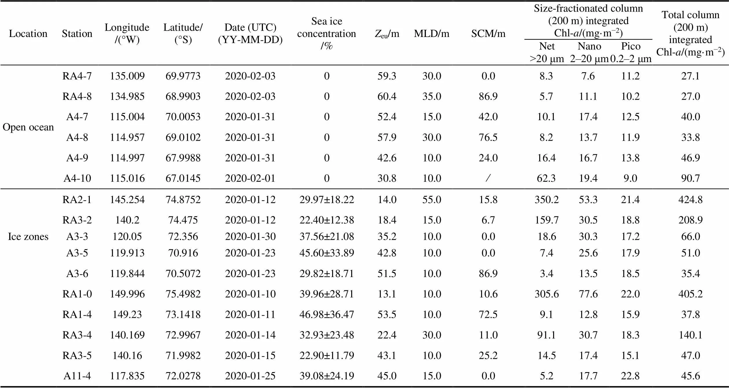
The western-Antarctic Amundsen Sea lies between Cape Flying Fish (the northwestern tip of Thurston Island) and Cape Dart, Siple Island. From 3 January to 5 February 2020 aboard the Chinese icebreaker R/V, samples from 46 size-fractionated Chl stations (Figure 1) from Amundsen polynya (AP), ice zones, and open ocean regions were collected. Polynya regions had sea-ice concentrations below 10% and were surrounded by ice (Arrigo and van Dijken, 2003). Two polynya regions (red dashed ellipses) were identified, with labelled dark dots indicating polynya stations (Figure 2). Sea-ice was absent in open-ocean stations. Data for sea-ice concentrations are derived from the Norwegian Meteorological Institute (https://osi-saf. eumetsat.int/products/sea-ice-products).

Figure 1 Amundsen Sea size-fractionated Chl-stations (dots) and transects (lines), 2020.

Figure 2 Sea ice concentration derived from the Norwegian Meteorological Institute. Dashed ellipses: red, polynya regions; black, open-ocean regions. Labeled dark dots indicate polynya stations.

2.2 Euphotic zone and mixed layer depths (MLDs)

We define the depth of the mixed layer as the depth at which the density is 0.05 kg·m−3higher than that of the sea surface (Brainerd and Gregg, 1995). The depth at which photosynthetically active radiation (PAR) is 1% that of surface PAR is defined as the euphotic zone depth (eu). Vertical light attenuation (d) for each station is calculated from the linear relationship established betweendand average Chl-concentrations (Morel et al., 2007).euis quantitatively related withd(Yang et al., 2015) as follows:

2.3 Size-fractionated Chl analyses and vertical distribution

Water samples for size-fractionated Chl were obtained for each station at 7 depths (0, 30, 50, 75, 100, 150, 200 m) using a CTD rosette sampler. Water samples (0.5–1 L) were filtered sequentially through 20 and 2 μm Nucleopore filters (47 mm) and Whatman GF/F filters (47 mm). Chl on filters was extracted in 90% acetone at −20°C for 24 h. Chl samples were measured onboard using a Trilogy fluorometer (Turner Designs, USA) (Holm-Hansen et al., 1965).

2.4 SCM analysis

SCM was obtained by fitting measured vertical Chl-data to a slightly modified version of the MB89 pattern (Uitz et al., 2006), using:

2.5 Data analysis

A Spearman correlation analysis was conducted to examine correlations between SCM and sea ice concentration,eu, MLD, and size-fractionated column-integrated Chl at survey stations. A Students-test was used to analyze for significant differences. Analyses were performed using SPSS 22.0.

3 Results

3.1 Euphotic zone and MLDs

euranged 11.3–24.3 m in the AP, 33.7–74.5 m in open ocean, and 13.1–53.5 m in ice zones (Table 1). Euphotic zone depth at AP stations were significantly lower than in open sea (test,< 0.01) and sea ice (test,< 0.05) stations because of higher Chl-concentrations.

MLD in AP, open ocean, and ice zones are detailed in Table 1. Because of stratification from melted sea ice or surface warming, MLD ranged 10–55 m at all stations. MLD in AP, open ocean, and ice zones did not differ significantly (test,> 0.05).

3.2 Total and size-fractionated Chl

Total column (200 m) integrated Chl (Figure 3) in AP stations ranged 167.6–766.3 mg·m−2(mean ± SD, 372.3 ± 189.0 mg·m−2), in open ocean stations 18.6–90.7 mg·m−2(49.0 ± 20.8 mg·m−2), and in ice zone stations 35.4– 424.8 mg·m−2(146.2 ± 152.1 mg·m−2). The highest and lowest integrated Chl values were 766.3 mg·m−2at station RA2-2 and 18.6 mg·m−2at station A3-8. Total column-integrated Chl in the AP was significantly higher than in open ocean (test,< 0.01) and ice zones (test,< 0.01). Total column-integrated Chl within ice zones was greater than in open ocean regions, but the difference was not significant (test,> 0.05). Highest Chl values occurred near shelf regions, especially at the southern ends of transects RA2 and A11.

Table 1 Amundsen Sea sea-ice concentration, Zeu, MLD, SCM, size-fractionated Chl, and total column integrated Chl

Continued

Figure 3 Total column-integrated Chl (0–200 m).

Column-integrated Chl (0–200 m, mg·m−2) values for netplankton (> 20 μm), nanoplankton (2–20 μm), and picoplankton (0.2–2 μm) in AP, open ocean, and ice zones are presented in Figure 4. Highest and lowest netplankton values were 590.9 mg·m−2at station RA2-2 and 1.8 mg·m−2at station A3-8, ranging 66.0–590.9 mg·m−2(233.6 ± 159.8 mg·m−2) in AP stations, 1.8–62.3 mg·m−2(19.0 ± 14.8 mg·m−2) in open ocean stations, and 3.4–350.2 mg·m−2(96.5 ± 132.3 mg·m−2) in ice zones (Figure 4a). Column-integrated netplankton Chl in AP stations was significantly higher than in open sea (test,< 0.01) and sea-ice (test,< 0.05) stations. The netplankton and total Chl-distributions were similar.

Highest and lowest nanoplankton Chl values were 140.6 mg·m−2at station A9-2 and 6.1 mg·m−2at station A3-8, ranging30.9–140.6 mg·m−2(75.9 ± 34.0 mg·m−2) in AP stations, 6.1–34.6 mg·m−2(15.9 ± 7.0 mg·m−2) in open ocean stations, and 12.8–77.6 mg·m−2(30.9 ± 20.3 mg·m−2) in ice zones (Figure 4b). Nanoplankton Chl in AP stations was significantly higher than in the open ocean (test,< 0.01) and ice zones (test,< 0.01). Column-integrated nanoplankton Chl in ice zones was significantly higher than in the open ocean regions (test,< 0.05).

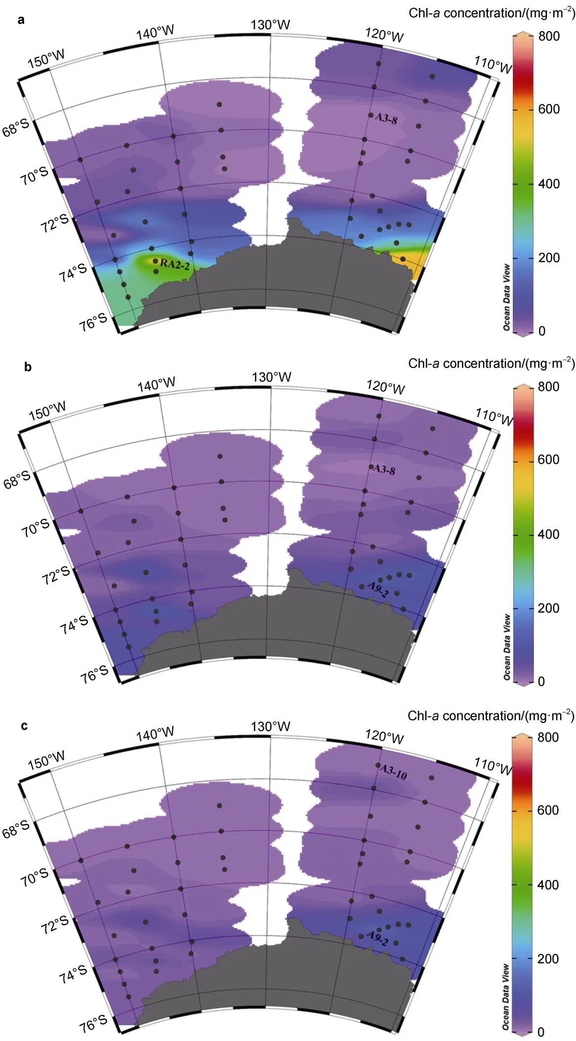
Figure 4 Column-integrated Chl (0–200 m) for netplankton (> 20 μm, a), nanoplankton (2–20 μm, b), and picoplankton (0.2–2 μm, c).

Highest and lowest integrated picoplankton Chl values were 173.9 mg·m−2at station A9-2 and 8.0 mg·m−2at station A3-10, ranging 16.3–173.9 mg·m−2(62.8 ± 42.0 mg·m−2) in AP stations, 8.0–32.7 mg·m−2(14.1 ± 5.3 mg·m−2) in open ocean stations, and 15.1–22.8 mg·m−2(18.8 ± 2.6 mg·m−2) in ice zones (Figure 4c). Picoplankton Chl in the AP was significantly higher than in the open ocean (test,< 0.01) and ice zones (test,< 0.01). Although the integrated picoplankton Chl in ice zones was similar to that of open ocean regions, they differed significantly (test,< 0.05).

Size-fractionated Chl indicates two distinctly different phytoplankton communities exist in the Amundsen Sea (Figure 5). In polynya, net-, nano-, and picoplankton cells comprise 63%, 20%, and 17% of the total Chl, respectively (Figure 5b).In ice zones, net-, nano-, and picoplankton cells comprise 63%, 23%, and 14% of the total Chl, respectively (Figure 5c). In contrast, the contribution to total Chl of net- (39%), nano- (32%), and picoplankton(29%) in open ocean stations was more evenly spread. The total phytoplankton community in the Amundsen Sea was dominated by netplankton, accounting for 60% of the total Chl, followed by nano-plankton (22%) and picoplankton (18%) (Figure 5a).

Figure 5 Size-fractionated Chl compositions in the overall Amundsen Sea (a), polynya (b), ice zones (c), and open ocean areas (d).

Chl-vertical distributions are shown in Figure 6. Maximum Chl occurs above 50 m, and decreases from 50–200 m Chl at all stations. Average Chl in the upper 50 m at AP stations, 4.9 ± 2.9 mg·m−3, was significantly higher than in ice zones (2.9 ± 3.4 mg·m−3,test,< 0.01) and open ocean stations (0.5 ± 0.4 mg·m−3,test,< 0.01). Intermediate average Chl values occurred in ice zones; open ocean stations had the lowest average Chl-concentration.

Chl-vertical distributions from 0–200 m along transects RA1–3, and A3 are presented in Figure 7. Maxima in the upper 50 m are associated with AP stations near the coast along all transects, and deep Chl-(> 50 m) are associated with AP station RA2-2 along transect RA2 (Figure 7b).

3.3 SCM

Chl-vertical profiles and corresponding modeled dimensionless Chl-profiles are shown in Figure 8. Measured Chl-vertical profiles were used in conjunction with equation (2), with the fitting procedure allowing the five parameters in this equation to be derived for each station (Table S1). Corresponding modeled dimensionless Chl-profiles compared well with measured Chl-vertical profiles for all stations (Figure 8). TheSCM ranged 0– 59.0 m (20.0 ± 16.5 m) in AP stations, 0–86.9 m (36.6 ± 28.6 m) in the open ocean, and 0–86.9 m (22.9 ± 31.2 m) in ice zones (Table 1). Average SCM values are lowest in the AP, followed by ice zones, then the open ocean.

SCM distributions along transects RA1 (a), RA2 (b), RA3 (c), and A3 (d) are presented in Figure 7. In polynya and ice zones near the shelf, the SCM was very low and generally remained at approximately 10 m. As the latitude decreases, in the open ocean, the SCM occurred deeper, excepting station RA1-5 on transect RA1, RA2-5 on transect RA2, and A3-10 on transect A3. Marginal ice zone stations RA1-5 and RA2-5, where sea ice melting released phytoplankton and iron, resulted in the SCM occurring in the upper water column, above the mixed layer. At station A3-10, physical processes such as eddies may have reintroduced the limiting micro-nutrient iron from depths into the upper water column, causing a phytoplankton bloom, lowering the SCM.

4 Discussion

4.1 Amundsen Sea Chl-a concentrations

Phytoplankton concentrations in the Amundsen Sea vary seasonally (Kim et al., 2015). Average column-integrated Chl from 0–30 m peaked in summer and decreased in winter (Smith et al., 1998). A comparison of dominant phytoplankton and Chl-concentrations throughout the Southern Ocean is presented in Table 2. Lee et al. (2012) reported high average Chl in polynya stations (395.1 ± 219.4 mg·m−2) compared to non-polynya stations (33.2 ± 23.9 mg·m−2) integrated from the surface to the bottom of the euphotic zone from 21 December 2010 to 23 January 2011. In contrast, Kim et al. (2016) reported a relatively low average Chl (49.2 mg·m−2) from 11 February to 14 March 2012. We report average Chl (372.32 ± 189.00 mg·m−2) from 3 January to 5 February 2020, column integrated from 0–200 m in polynya, being twice higher than in ice zones (146.17 ± 152.07 mg·m−2) and seven times higher than in open ocean areas (48.95 ± 20.82 mg·m−2). Ouraverage Chl in polynya areas is within the range reported by Lee et al. (2012), but significantly higher in non-polynya areas, possibly due to different integrated depths between studies (～ 50 m in the euphotic zone in Lee et al. (2012), but 200 m herein).

4.2 Amundsen Sea phytoplankton composition

Phytoplankton community structure can significantly affect trophic levels, phytoplankton biochemical composition, and particulate organic carbon transfer efficiency in pelagic food chains (Harrison et al., 1990; Lee et al., 2007; Cotti-Rausch et al., 2020). While the biomass of phytoplankton of given sizes can affect food webs, the activity of size fractions is more directly relevant to trophic dynamics and biogeochemical cycling (Cotti-Rausch et al., 2020). At higher ammonium concentrations (～ 5 μM) in the Chukchi Sea and Bering Strait, small phytoplankton (< 5 μm) incorporate more carbon into proteins than larger phytoplankton (> 5 μm) (Lee et al., 2009). We reported netplankton (> 20 μm) to dominate (63%) in polynya and ice zones, possibly because ofblooms in seasonal ice zones and coastal Antarctic waters (DiTullio et al., 2000). In contrast, with decreased latitude, the proportion of netplankton gradually decreases and that of nano- and picoplankton increases. The three size-fractionated phytoplankton groups are more evenly distributed in open ocean stations, possibly because of iron limitation inhibiting uptake of major macronutrients by phytoplankton (Peloquin and Smith, 2007).

Figure 6 Chl-vertical distributions in polynya (a), ice zone (b), and open ocean (c) stations.

Figure 7 Chl-distributions from 0–200 m along transects RA1 (a), RA2 (b), RA3 (c), and A3 (d). Dashed lines: black, MLD; orange, SCM.

Figure 8 Chl-vertical profiles and corresponding modeled dimensionless Chl-profiles at polynya (a), ice zone (b), and open-ocean (c) stations.

4.3 Amundsen Sea subsurface chlorophyll maxima

The stability of the tropical SCM relies on the vertical mixing input of limiting nutrients that enter the base of the mixed layer through the pycnocline, combined with a light field that decreases exponentially with depth (Latasa et al., 2017). This creates an optimum depth for phytoplankton to grow (at the SCM), usually just above the pycnocline (Baldry et al., 2020). Unalike tropical regions, sufficient subsurface inputs of iron, the limiting micro-nutrient, are not widely present in the Southern Ocean (Arteaga et al., 2019). The Southern Ocean SCM is influenced by various processes, such as iron fertilization from land masses, sea-ice retreat, eddies, buoyancy regulation by large diatoms, and grazing (Ardyna et al., 2019). In Amundsen Sea polynya and ice edge areas, sea-ice retreat releases phytoplankton, alleviates light limitation, and increases bioavailable iron concentrations with the melting of ice, resulting in surface water phytoplankton blooms. Around the Amundsen Sea shelf, the continuous supply of iron from ocean depths because of the Antarctic Circumpolar Current promotes large-scale phytoplankton blooms dominated by diatoms (netplankton, > 20 μm) in surface waters. The Amundsen Sea SCM is moderately, positively correlated witheu, and moderately, negatively correlated with column-integrated net- and nanoplankton Chl (Table 3). With diatom blooms,eudecreases and diatom SCMs occur in surface blooms, above the pycnocline. The diatom SCM forms under continuous iron or silicate limiting conditions with the reduction of surface blooms (Gomi et al., 2007).When nutrients from meltwater are rapidly depleted, the net- and nanoplankton column-integrated Chl gradually decreases and the surface bloom at the sea ice edge sinks rapidly. Sinking phytoplankton find an appropriate environment deeper than the pycnocline, aggregating to form a SCM in the Amundsen Sea open ocean.

5 Summary and conclusions

Average column-integrated (0–200 m) Chl from 3 January to 5 February 2020 in the Amundsen polynya ranged 372.3 ± 189.0 mg·m−2, consistent with values reported by Lee et al. (2012) for average Chl integrated from surface to the bottom of the euphotic zone in polynya regions. However, our average Chl in non-polynya areas is significantly higher than that reported by Lee et al. (2012). Phytoplankton communities in Amundsen Sea polynya and ice zones are dominated by netplankton, which accounts for 60% of the total Chl because ofblooms (DiTullio et al., 2000). Diatom SCMs are located in surface blooms, above the pycnocline. In contrast, net-, nano-, and picoplankton contribute more evenly to total Chl in open-ocean stations, likely because of iron limitation. In the open ocean, because of iron and light colimitation, the SCM migrates deeper and occurs below the pycnocline. The Amundsen Sea SCM is moderately correlated witheuand column-integrated net- and nanoplankton Chl. In the Amundsen Sea, sea-ice concentrations decrease by about 7% per decade (Cavalieri and Parkinson, 2008). To better understand the mechanisms driving significant differences in Chl, phytoplankton composition, and SCM depths among polynya and non-polynya areas in the Amundsen Sea, more seasonal and annual surveys are required.

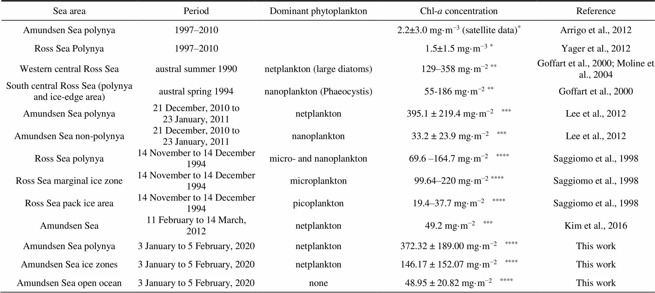
Table 2 Comparison of dominant phytoplankton and Chl-a concentrations in the Southern Ocean

Notes: * mean Chl-concentration from satellite data; ** column-integrated Chl-concentration in the upper 100 m; *** column-integrated Chl-concentration from surface to the bottom of the euphotic zone; **** column-integrated Chl-concentration in the upper 200 m.

Table 3 Correlations between the SCM and environmental parameters

Notes: *< 0.05, **< 0.01.

Acknowledgments We thank the captain, Bing Zhu and crew of R/V, and Mr. Shuo He from Zhejiang University for their assistance during sampling. This research was financially supported by National Polar Special Program “Impact and Response of Antarctic Seas to Climate Change” (Grant no. IRASCC 01-02-01).We appreciate two anonymous reviewers, and Guest Editor Prof. Rujian Wang for their constructive comments that have further improved the manuscript.

Note Zhang Wei and Hao Qiangcontributedequallytothisworkandshouldbeconsideredco-firstauthors.

Ardyna M, Lacour L, Sergi S, et al. 2019. Hydrothermal vents trigger massive phytoplankton blooms in the Southern Ocean. Nat Commun, 10(1), 2451, doi:10.1038/s41467-019-09973-6.

Arrigo K R, van Dijken G L. 2003. Phytoplankton dynamics within 37 Antarctic coastal polynya systems. J Geophys Res, 108(C8): 3271, doi:10.1029/2002jc001739.

Arrigo K R, Lowry K E, van Dijken G L. 2012. Annual changes in sea ice and phytoplankton in polynyas of the Amundsen Sea, Antarctica. Deep Sea Res Part II Top Stud Oceanogr, 71-76: 5-15, doi:10.1016/ j.dsr2.2012.03.006.

Arrigo K R, Robinson D H, Worthen D L, et al. 1999. Phytoplankton community structure and the drawdown of nutrients and CO2in the Southern Ocean. Science, 283(5400): 365-367, doi:10.1126/science. 283.5400.365.

Arteaga L A, Pahlow M, Bushinsky S M, et al. 2019. Nutrient controls on export production in the Southern Ocean. Global Biogeochem Cycles, 33(8): 942-956, doi:10.1029/2019gb006236.

Baldry K, Strutton P G, Hill N A, et al. 2020. Subsurface chlorophyll-maxima in the Southern Ocean. Front Mar Sci, 7: 671, doi:10.3389/ fmars.2020.00671.

Brainerd K E, Gregg M C. 1995. Surface mixed and mixing layer depths. Deep Sea Res Part I Oceanogr Res Pap, 42(9): 1521-1543, doi:10.1016/0967-0637(95)00068-H.

Caron D A, Dennett M R, Lonsdale D J, et al. 2000. Microzooplankton herbivory in the Ross Sea, Antarctica. Deep Sea Res Part II Top Stud Oceanogr, 47(15-16): 3249-3272, doi:10.1016/S0967-0645(00)00067- 9.

Cavalieri D J, Parkinson C L. 2008. Antarctic sea ice variability and trends, 1979–2006. J Geophys Res, 113(C7): C07004, doi:10.1029/2007jc 004564.

Cotti-Rausch B E, Lomas M W, Lachenmyer E M, et al. 2020. Size-fractionated biomass and primary productivity of Sargasso Sea phytoplankton. Deep Sea Res Part I Oceanogr Res Pap, 156: 103141, doi:10.1016/j.dsr.2019.103141.

Deppeler S L, Davidson A T. 2017. Southern Ocean phytoplankton in a changing climate. Front Mar Sci, 4: 1-28, doi:10.3389/fmars.2017. 00040.

DiTullio G R, Grebmeier J M, Arrigo K R, et al. 2000. Rapid and early export ofblooms in the Ross Sea, Antarctica. Nature, 404(6778): 595-598, doi:10.1038/35007061.

Fragoso G M, Smith W O. 2012. Influence of hydrography on phytoplankton distribution in the Amundsen and Ross Seas, Antarctica. J Mar Syst, 89(1): 19-29, doi:10.1016/j.jmarsys.2011.07.008.

Goffart A, Catalano G, Hecq J H. 2000. Factors controlling the distribution of diatoms and Phaeocystis in the Ross Sea. J Mar Syst, 27(1-3): 161-175, doi:10.1016/S0924-7963(00)00065-8.

Gomi Y, Taniguchi A, Fukuchi M. 2007. Temporal and spatial variation of the phytoplankton assemblage in the eastern Indian sector of the Southern Ocean in summer 2001/2002. Polar Biol, 30(7): 817-827, doi:10.1007/s00300-006-0242-2.

Harrison P J, Thompson P A, Calderwood G S. 1990. Effects of nutrient and light limitation on the biochemical composition of phytoplankton. J Appl Phycol, 2(1): 45-56, doi:10.1007/BF02179768.

Holm-Hansen O, Lorenzen C J, Holmes R W, et al. 1965. Fluorometric determination of chlorophyll. J Mar Sci, 30: 3-15, doi:10.1093/ icesjms/30.1.3.

Jacobs S S, Jenkins A, Giulivi C F, et al. 2011. Stronger ocean circulation and increased melting under Pine Island Glacier ice shelf. Nat Geosci, 4(8): 519-523, doi:10.1038/ngeo1188.

Kim B K, Joo H, Song H J, et al. 2015. Large seasonal variation in phytoplankton production in the Amundsen Sea. Polar Biol, 38(3): 319-331, doi:10.1007/s00300-014-1588-5.

Kim B K, Lee J H, Joo H, et al. 2016. Macromolecular compositions of phytoplankton in the Amundsen Sea, Antarctica. Deep Sea Res Part II Top Stud Oceanogr, 123: 42-49, doi:10.1016/j.dsr2.2015.04.024.

Latasa M, Cabello A M, Morán X A G, et al. 2017. Distribution of phytoplankton groups within the deep chlorophyll maximum. Limnol Oceanogr, 62(2): 665-685, doi:10.1002/lno.10452.

Lee, S H, Kim B K, Yun M S, et al. 2012. Spatial distribution of phytoplankton productivity in the Amundsen Sea, Antarctica. Polar Biol, 35: 1721-1733, doi:10.1007/s00300-012-1220-5.

Lee S H, Kim H J, Whitledge T E. 2009. High incorporation of carbon into proteins by the phytoplankton of the Bering Strait and Chukchi Sea Cont Shelf Res, 29(14): 1689-1696, doi:10.1016/j.csr.2009.05.012.

Lee S H, Whitledge T E, Kang S H. 2007. Recent carbon and nitrogen uptake rates of phytoplankton in Bering Strait and the Chukchi Sea. Cont Shelf Res, 27(17): 2231-2249, doi:10.1016/j.csr.2007. 05.009.

Liss P S, Malin G, Turner S M, et al. 1994. Dimethyl sulphide and: a review. J Mar Syst, 5(1): 41-53, doi:10.1016/0924- 7963(94)90015-9.

Moline M A, Claustre H, Frazer T K, et al. 2004. Alteration of the food web along the Antarctic Peninsula in response to a regional warming trend. Glob Change Biol, 10(12): 1973-1980, doi:10.1111/j.1365-2486. 2004.00825.x.

Morel A, Huot Y, Gentili B, et al. 2007. Examining the consistency of products derived from various ocean color sensors in open ocean (Case 1) waters in the perspective of a multi-sensor approach. Remote Sens Environ, 111(1): 69-88, doi:10.1016/j.rse.2007.03.012.

Peloquin J A, Smith W O. 2007. Phytoplankton blooms in the Ross Sea, Antarctica: Interannual variability in magnitude, temporal patterns, and composition. J Geophys Res, 112(C8): C08013, doi:10.1029/ 2006jc003816.

Rignot E, Bamber J L, van den Broeke M R, et al. 2008. Recent Antarctic ice mass loss from radar interferometry and regional climate modelling. Nat Geosci, 1 (2): 106-110, doi:10.1038/ngeo102.

Saggiomo V, Carrada G C, Mangoni O, et al. 1998. Spatial and temporal variability of size-fractionated biomass and primary production in the Ross Sea (Antarctica) during austral spring and summer. J Mar Syst, 17(1-4): 115-127, doi:10.1016/S0924-7963(98)00033-5.

Sarmiento J L, Slater R, Barber R, et al. 2004. Response of ocean ecosystems to climate warming. Global Biogeochem Cycles, 18(3): GB3003, doi:10.1029/2003gb002134.

Siegelman L, O’Toole M, Flexas M, et al. 2019. Submesoscale ocean fronts act as biological hotspot for southern elephant seal. Sci Rep, 9(1), 5588, doi:10.1038/s41598-019-42117-w.

Smith R C, Baker K S, Vernet M. 1998. Seasonal and interannual variability of phytoplankton biomass west of the Antarctic Peninsula. J Mar Syst, 17(1-4): 229-243, doi:10.1016/s0924-7963(98)00040-2.

Smith Jr. W, Barber D. 2007. Polynyas: windows to the world. Elsevier.

Strzepek R F, Boyd P W, Sunda W G. 2019. Photosynthetic adaptation to low iron, light, and temperature in Southern Ocean phytoplankton. PNAS, 116(10): 4388-4393, doi:10.1073/pnas.1810886116.

Tripathy S C, Pavithran S, Sabu P, et al. 2015. Deep chlorophyll maximum and primary productivity in Indian Ocean sector of the Southern Ocean: Case study in the Subtropical and Polar Front during austral summer 2011. Deep Sea Res Part II Top Stud Oceanogr, 118: 240-249, doi:10.1016/j.dsr2.2015.01.004.

Uitz J, Claustre H, Morel A, et al. 2006. Vertical distribution of phytoplankton communities in open ocean: An assessment based on surface chlorophyll. J Geophys Res, 111(C8): C08005, doi:10.1029/ 2005jc003207.

Yager P, Sherrell R, Stammerjohn S, et al. 2012. ASPIRE: The Amundsen Sea polynya international research expedition. Oceanography, 25(3): 40-53, doi:10.5670/oceanog.2012.73.

Yang W, Matsushita B, Yoshimura K, et al. 2015. A modified semianalytical algorithm for remotely estimating euphotic zone depth in Turbid Inland waters. IEEE Journal of Selected Topics in Applied Earth Observations and Remote Sensing, 8: 1-10, doi:10.1109/ JSTARS.2015.2415853.

Table S1 Values of the five parameters to be used in equation (7) obtained for the dimensionless vertical profiles of Chl-and subsurface chlorophyll maximum (SCM) for all stations in the Amundsen Sea polynya, ice zones, and open ocean

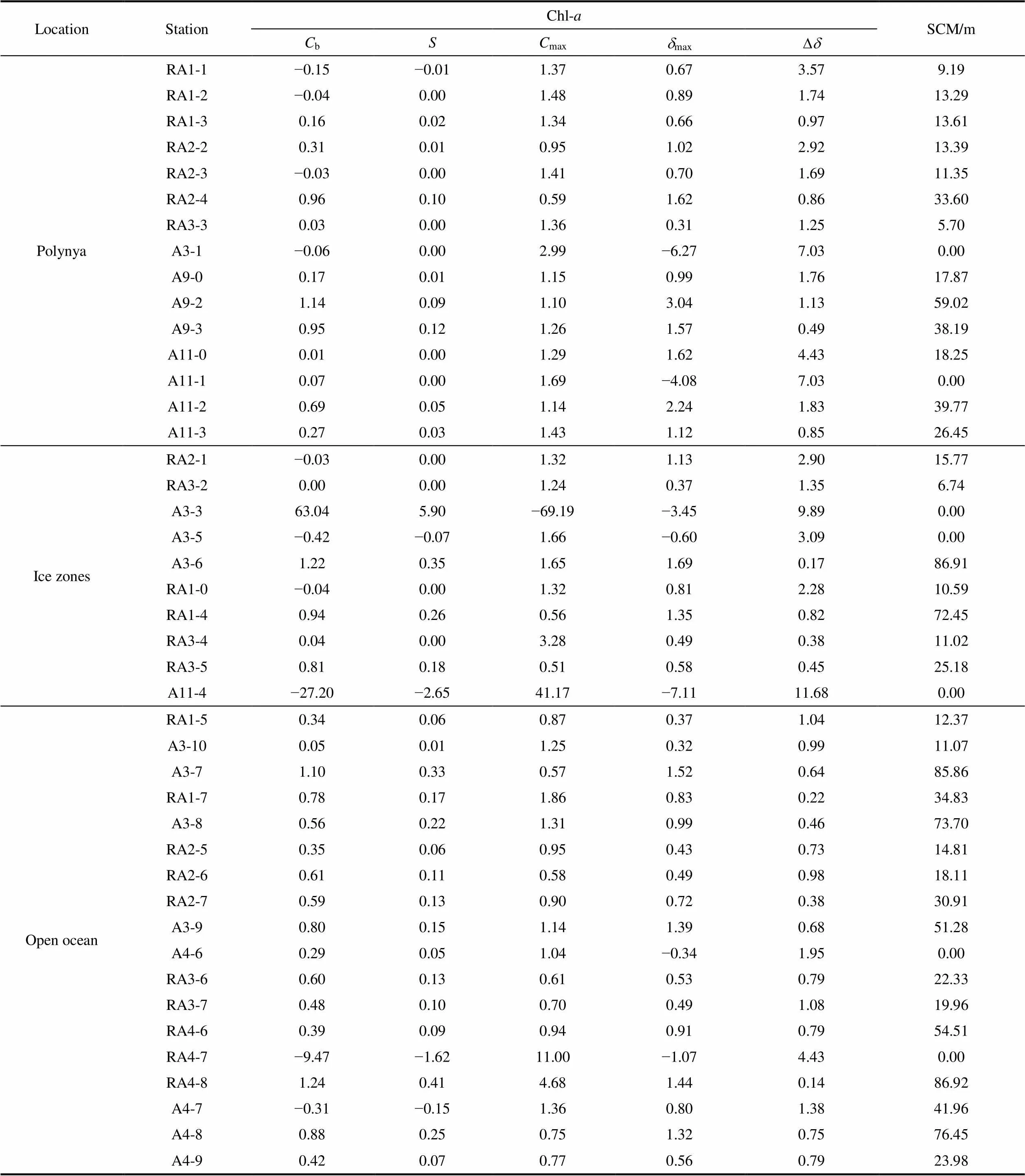
LocationStationChl-aSCM/m CbSCmaxdmaxDd PolynyaRA1-1−0.15−0.011.370.673.579.19 RA1-2−0.040.001.480.891.7413.29 RA1-30.160.021.340.660.9713.61 RA2-20.310.010.951.022.9213.39 RA2-3−0.030.001.410.701.6911.35 RA2-40.960.100.591.620.8633.60 RA3-30.030.001.360.311.255.70 A3-1−0.060.002.99−6.277.030.00 A9-00.170.011.150.991.7617.87 A9-21.140.091.103.041.1359.02 A9-30.950.121.261.570.4938.19 A11-00.010.001.291.624.4318.25 A11-10.070.001.69−4.087.030.00 A11-20.690.051.142.241.8339.77 A11-30.270.031.431.120.8526.45 Ice zonesRA2-1−0.030.001.321.132.9015.77 RA3-20.000.001.240.371.356.74 A3-363.045.90−69.19−3.459.890.00 A3-5−0.42−0.071.66−0.603.090.00 A3-61.220.351.651.690.1786.91 RA1-0−0.040.001.320.812.2810.59 RA1-40.940.260.561.350.8272.45 RA3-40.040.003.280.490.3811.02 RA3-50.810.180.510.580.4525.18 A11-4−27.20−2.6541.17−7.1111.680.00 Open oceanRA1-50.340.060.870.371.0412.37 A3-100.050.011.250.320.9911.07 A3-71.100.330.571.520.6485.86 RA1-70.780.171.860.830.2234.83 A3-80.560.221.310.990.4673.70 RA2-50.350.060.950.430.7314.81 RA2-60.610.110.580.490.9818.11 RA2-70.590.130.900.720.3830.91 A3-90.800.151.141.390.6851.28 A4-60.290.051.04−0.341.950.00 RA3-60.600.130.610.530.7922.33 RA3-70.480.100.700.491.0819.96 RA4-60.390.090.940.910.7954.51 RA4-7−9.47−1.6211.00−1.074.430.00 RA4-81.240.414.681.440.1486.92 A4-7−0.31−0.151.360.801.3841.96 A4-80.880.250.751.320.7576.45 A4-90.420.070.770.560.7923.98

10.13679/j.advps.2021.0035

12 July 2021;

26 October 2021;

30 March 2022

: Zhang W, Hao Q, He J F, et al.Variability of size-fractionated phytoplankton standing stock in the Amundsen Sea during summer. Adv Polar Sci, 2022, 33(1): 1-13,doi:10.13679/j.advps.2021.0035

, ORCID: 0000-0003-2145-2703, E-mail: haoq@sio.org.cn