Robust function-on-function regression model with nonparametric random effects

Shanshan Wang,Hao Ding ,and Zhanfeng Wang

Department of Statistics and Finance,School of Management,University of Science and Technology of China,Hefei 230026,China

Abstract: Extended t-process is robust to outliers and inherits many attractive properties from the Gaussian process.In this paper,we provide a function-on-function nonparametric random-effects model using extended t-process priors in which we consider heterogeneity of individual effect,flexible mean function,nonparametric covariance function and robustness.A likelihood-based estimation procedure is constructed to estimate parameters involved in the model.Information consistency for the parameter estimation is provided.Simulation studies and a real data example are further investigated to evaluate the performance of the developed procedures.

Keywords: extended t-process regression;nonlinear random effects;covariance kernel function;robustness

1 Introduction

As the development of science and technology,some data sets are recorded frequently with curves,surfaces and other types,which are usually called functional data that plays an important role in wide fields such as atmospheric science,engineering,medical research,see more details in Ramsay and Silverman[1].Functional regression models are useful tools in functional data analysis,where one of the most interesting and challenging cases is function-on-function regression,see Ramsay and Silverman[1,2],Yao et al.[3,4].In this paper,we consider the following functional model proposed by Wang et al.[5],form=1,···,M,

whereym(t)is the functional response,zm(t)is ap-vector of functional covariates,νis the corresponding parameters,xm(s,t)is aq-dimensional of covariatesdepends onsandt,a nd β(s,t)is a vector of the functional coefficients,Stis interval fort,εm(t)is random error term for themth curve.Model(1) is flexible,and includes some function-on-function models in Gervini[6],Malfait and Ramsay[7],Ramsay and Silverman[2],as special cases.Note thatτmisused to model the heterogeneity among the different subjects,which depends onzm(t),xm(·,t).Wang et al.[5]considered the above random effects model using Gaussian process priors.More on Gaussian process priors in functional model[8,9].

However,when there exist outliers in the observations,it is not robust to use the model based on Gaussian process priors,see e.g.Wang et al.[10].Then in order to overcome the influence of outliers,various forms of student t-process have been developed to model a heavy-tailed process,e.g.Yu et al.[11],Zhang and Yeung[12].Shah et al.[13]pointed out that the t-distribution under addition is not closed to maintain the good properties of Gaussian models.Thus,Wang et al.[10]developed an extendedt-process regression,which has the following advantages:①it can maintain the good properties of Gaussian process;② it has flexible forms,and contains model in Shah et al.[13]as a special case;③it is robust.More general discussions ont-process can see Refs.[10,14].

In this paper,we consider a functional nonparametric random effects model with extended t-process priors,and propose an estimation procedure.The proposed method has 3 merits.①It applies the extendedt-process prior to model the heterogeneity of individual effect in the function-on-function regression model such that the model has robustness;② A basis expansion smoothing method and a penalized likelihood method are developed to estimate the parameter in the fixed effect and covariance function of random effects,which leads to estimation of the smoothing function and prediction of the random effect;③Information consistency of the parameter estimation is obtained.

The remainder of the paper is organized as follows.In Section 2,we present the nonparametric random effects model using extendedt-process priors,and develop prediction distribution and estimation procedure.In Section 3,we conduct simulation studies and a real data example to evaluate the performance of the proposed method.The conclusions are given in Section 4.All the proofs are given in Appendix.

2 Main results

2.1 Extended t-process

Extendedt-process proposed by Wang et al.[10]is briefly introduced as follows.Letf(·),a real-valued random function from X toR,satisfy that

where GP(·,·) and IG(·,·) stand for Gaussian process and inverse gamma distribution respectively.Thenffollows an extendedt-process (ETP),and can be denoted byf～ETP(v,ω,h,k).We callh(·):X →Rmean function andk(·,·):X×X→Rcovariance kernel function.From the definition of ETP,we show that for any pointsX=(x1,···,xn)⊤,we have

meaning thatf nhas an extended multivariatet-distribution

(EMT D)with thef ollowing density function,

2.2 Function-on-function regression model with random effects

In model (1),the random effect τmdepicts individual effect.Considering robustness against outliers,an ETP process prior is applied toτm.This paper assumes that τmand εmhave a joint extendedt-process,

where δε(t,s)=I(t=s) andI(·) is an indicator function.

Note that the random effect τmrelies onzm(t) andxm(·,t),then following Wang et al.[5],the kernel functionkis an expression as

Let observations {ymi=ym(ti),i=1,···,n,m=1,···,M},error termwhere {ti} are observed times.Assume that true values of ν,β,τmin model(1) arerespectively.From model (1),we further consider the following (true) data model:

This paper aims to develop methods to estimate ν0,β0,and predict τ0m.

2.3 Prediction

It follows that for the observed data,we have the conditional distributions,

Denoted by the data set D={(ym(tj),um(tj)):j=1,···,n,m=1,···,M}.Sincethat

we obtain the posterior distribution of τm,that is

wherev*=v+n/2,w*=w+n/2,

and

For prediction,at a new data pointt*,we have

wherekmt=(k(um(t),um(t1)),···,k(um(t),um(tn)))⊤.It indicates that

where

Therefore,we can use posterior mean

to predictym(t*),denoted byAnd using

Similarly,

It follows that Eq.(4) is an estimation of the covariance function of

2.4 Parameter estimation

Note that β(s,t) in model (1) is a smooth function and can be approximated based on basis functions {ϕk(s),k=1,···,Ks},and{ψk(s),k=1,···,Kt},

where“ ⊗”represents the Kronecker product.Hence,

Next we estimate θ,band σ2via using a likelihood method.By Eq.(3),we obtain a likelihood function ofym,

Due to the smoothness of β(·,·),following from Ramsay and Silverman[5],we consider the following penalty functions,

where

Therefore,we develop an objective function,

whereλsand λtare tuning parameters.Take the derivative ofG(θ,b,σ2)with respect tob,we can obtain the estimation equation

where Λ=diag(0p×p,λs Jψψ⊗Lϕϕ+λt Lψψ⊗Jϕϕ,···,λs Jψψ⊗Lϕϕ+λt Lψψ⊗Jϕϕ)is a(p+qKsKt)×(p+qKsKt)matrix.Similarly,we can get estimation equations with respect to θ and σ2.

From these estimation equations,we construct an estimation procedure as follows.

Step 1 Given an initial estimate of θ;

Step 2 Given θ,we update the estimates ofband σ2via

Step 3 Givenband σ2,we update the estimate of θ via

Step 4 Repeat Step 2 and Step 3 until convergence.

Similar to Ref.[5],when the absolute value of relative difference ofl(θ,b,σ2) between two successive iterations is less than a given value,the procedure stops.

2.5 Information consistency

The common mean structure and its properties have been studied a lot in functional models,see Yao et al.[4],Yuan and Cai[15],Sun et al.[16],and among others.Next we only consider the information consistency.Let X=X1×X2,where X1and X2are spaces covariatesz m(t)andx m(·,t) belonging to.Letpσ0(ym|τ0m,um)be the density function to generate the dataymgivenumandτ0m,whereσ0is the true value of σ,τ0mis the t rue value ofτm.Letpθ(τ)be a measurement of the random processτon space F={τ(·,·):X→R}.Let

be the density function to generate the dataymgivenumunder model (1).Letbe the estimated density function.Denote

as the Kullback-Leibler divergence between two densitiesp1andp2.According to Ref.[6],we only need to show the Kullback-Leibler divergence between two density functions forym|umfrom the true and the assumed models tends to zero whennis largeenough.

For information consistency of the parameter estimation,we need the following condition.

Condition (A):‖ τ0m‖kis bounded and

where‖τ0m‖kis the reproducing kernel Hilbert space norm of τ0massociated withk(·,·;θ),Kmis covariance matrix ofτ0moverum,Iisthen×nidentity matrix.

More details about Condition (A)can see Seeger et al.[17]and Wang et al.[5].More on reproducing kernel Hilbert space can see Berlinet and Thomas[18].

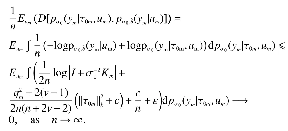
Proposition 2.1.Under the conditions in Lemma A.1 (Appendix) and condition (A),we have

where the expectation is taken over the distribution ofum.

3 Numerical results

3.1 Simulations

Performance of the proposed method is investigated by numerical studies.Simulation data are generated by the following model,

wherezm(·)～GP(h1,k1),h1=h1(t)=t,fort∈(0,1),k1=k1(zm(t1),zm(t2))=g(t1,t2)=0.1exp{-5(t1-t2)2}+0.1t1t2,andxm(·,·)～GP(h2,k2),h2=h2(t)=t+cos(s)(s),fort,s∈(0,1),k2=k2(xm(s1,t),xm(s2,t))=g(s1,s2).Letν=1.0,θ10=θ12=θ21=θ22=0.1,θ11=10,σ2=0.5,andtandstake 20 points equally in(0,1).Consider four different combinations ofτmand β(s,t),

S1:τm～GP(0,Cov(τm(um(t1)),τm(um(t2)))),andh2=h2(t)=t+cos(s)(s),fors,t∈(0,1);

S2:τm～GP(0,Cov(τm(um(t1)),τm(um(t2)))),andβ(s,t)=exp{-(t2+s2)}/10,fors,t∈(0,1);

S3:τm=0 and β (s,t)=(t2+cos(s))/10,fors,t∈(0,1);

S4:τm=0 and β (s,t)=exp{-(t2+s2)}/10,fors,t∈(0,1).

We take sample sizesM=10,20,and 30.All simulations are repeated 500 times.

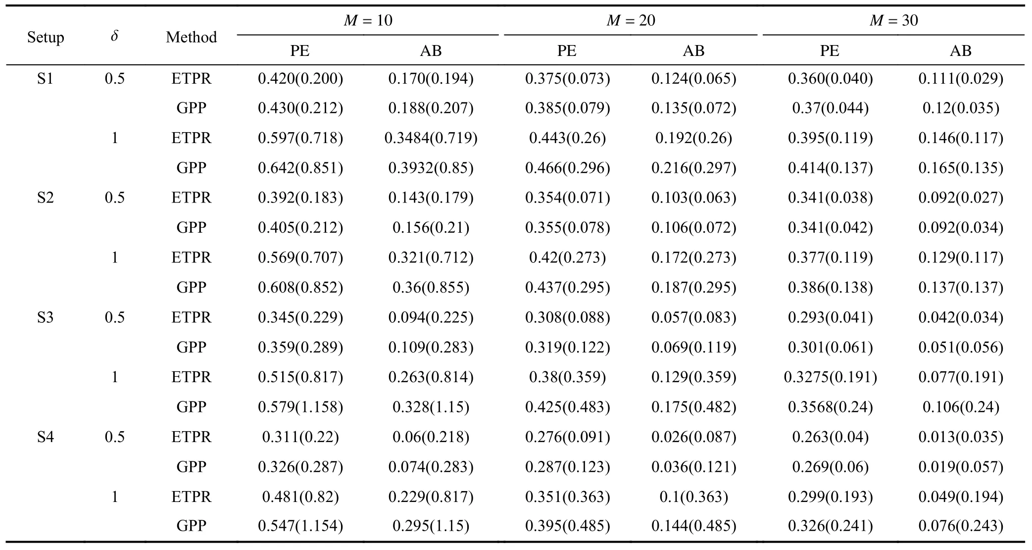
To show robustness of model (1) with random effect having ETPR,saying ETPR,we also compute model (1) with random effect having GPR,denoted by GPR.Two indices:prediction error (PE),

and average estimation bias (AB)

are applied to show performance of two methods:ETPR and GPR,whereis an estimator of the true regression functionf0(t)=To show robustness of our method,one curve is randomly selected and added with an extradisturbance,δt3,wheret3stands for studenttdistribution with degree of freedom 3.Table 1 presents the values of PE and AB from these two methods.We see that ETPR has smaller PE and AB than GPR,especially with δ=1.0 and small sample sizes.It shows that the proposed method ETPR has more robustness against outliers compared to GPR.

In addition,we also consider one constant disturbance for the abnormal curves with small sample sizes 10 and 20.Tables 2 and 3 present PE and AB of prediction from ETPR method and GPR method for one and two curves disturbed,respectively.We see that ETPR has better performance in prediction compared to GPR.

3.2 Real data example

The proposed method is applied to Canadian weather data,which is obtained from theRpackagefda.We aim to study fixed effect of temperature on precipitation by common temperature effect of stations in the same region,and random effect of temperature on precipitation by individual effect of each station.Generally,the 35 stations are divided into four regions:Arctic,Atlantic,Pacific and Continental.Obviously,there exists heterogeneity among the stations due to the spatial nature of the weather data.Then we propose the following model:

whereyij(t)represents precipitation andxij(t)represents temperature,for timet,regioniandjth station.In this model,we havezij(t)=1 andxij(s,t)=xij(s) which effectively simplifies mo del fit.

Table 1.PE and AB of prediction from ETPR method and GPR method,where SDs are presented in parentheses.

Table 2.PE and AB of prediction from ETPR method and GPR method with one curve disturbed by constant 1.0,where SDs are presented in parentheses.

Table 3.PE and AB of prediction from ETPR method and GPR method with two curves disturbed by constant 1.0,where SDs are presented in parentheses.

Fig.1.Random and fixed effects of model using ETPR for Arctic and Atlantic.

Fig.2.Random and fixed effects of model using ETPR for Continental and Pacific.

Figs.1 and 2 show random and fixed effects of the 4 regions:Arctic,Atlantic,Pacific and Continental from the proposed method.We see from the random effects that each station in the same region has different temperature effects on the precipitation.To compare performance of prediction from ETPR with GPR,10-folds cross validation method is used to compute mean squares of prediction errors,0.310 and 0.314,for ETPR and GPR,respectively.It shows that ETPR has a little better performance in prediction.

4 Conclusions

A function-on-function random effects model with extended tprocess prior in this paper is developed to analyze functional data which may include outliers.The proposed model is flexible,including various kinds of functional models,such as the function-on-function linear model[2]and the historical functional regression model[7]as special cases.The proposed extended t-process model is not only robust against outliers,but also inherits almost all the nice properties from Gaussian process regression,such as closed form of prediction and convenient computation procedure.The estimation procedure and computing algorithm are developed to estimate the parameters and predict the random effect in the regression model.The functional response considered in this paper has one dimension.In practical application,functional multi-response may consist of several correlated curves.It is interesting that the proposed method is extended to functional data with multi-response,which will be studied in our further work.

Appendix

LemmaA.1.Letw=v-1.Under model(1),assume thatym

are independently sampled,the covariance kernel functionkis bounded and continuous on the parameter θ,and θˆ converges to θ whenn→∞.Then,for a positive constantcand any ε ＞0,whennis large enough,we have

ProofofLemmaA.1.Assumerisa random variable fol-

lowing inverse gamma distribution IG(v,(v-1)).Conditional onr,we have

where GP(h,k) stands for Gaussian process with mean functionhand covariance functionk.Then conditional onr m,the extended t-process regression modelbecomes Gaussian process regression model

By similar procedures in Seeger et al.[17]and Wang et al.[10],for any givenr,we have

then it follows that

Letg*(r)be the density function of IG(v+n/2,v-1+It easily shows that

We have

which shows that Lemma A.1 holds.

Proof ofProposition 2.1.ObviouslyUnder the con ditions of Lemma A.1 and condition(A),by Lemma A.1,for a positive constantcand any ε ＞0,whennis large enough,we have

Thus,it completes the proof.

Acknowledgements

We thank the reviewers for their insightful comments and suggestions.This work was supported in part by the National Natural Science Foundation of China (11971457),Anhui Provincial Natural Science Foundation (1908085MA06) and the Fundamental Research Funds for the Central Universities(WK2040000035).

Conflict of interest

The authors declare that they have no conflict of interest.

Biographies

Shanshan Wangis currently a master student under the supervision of Assoc.Prof.Zhanfeng Wang at the University of Science and Technology of China.Her research mainly focuses on functional data.

Hao Dingreceived his PhD degree from the University of Science and Technology of China (USTC).He is currently a postdoctoral fellow at USTC.His research focuses on robust estimation,functional data analysis.