A Personalized Comprehensive Cloud-Based Method for Heterogeneous MAGDM and Application in COVID-19

Xiaobing Mao,Hao Wu and Shuping Wan

School of Information Management,Jiangxi University of Finance and Economics,Nanchang,330013,China

ABSTRACT This paper proposes a personalized comprehensive cloud-based method for heterogeneous multi-attribute group decision-making(MAGDM),in which the evaluations of alternatives on attributes are represented by LTs(linguistic terms),PLTSs (probabilistic linguistic term sets) and LHFSs (linguistic hesitant fuzzy sets).As an effective tool to describe LTs,cloud model is used to quantify the qualitative evaluations.Firstly,the regulation parameters of entropy and hyper entropy are defined,and they are further incorporated into the transformation process from LTs to clouds for reflecting the different personalities of decision-makers(DMs).To tackle the evaluation information in the form of PLTSs and LHFSs,PLTS and LHFS are transformed into comprehensive cloud of PLTS(C-PLTS)and comprehensive cloud of LHFS(C-LHFS),respectively.Moreover,DMs’weights are calculated based on the regulation parameters of entropy and hyper entropy.Next,we put forward cloud almost stochastic dominance(CASD) relationship and CASD degree to compare clouds.In addition,by considering three perspectives,a comprehensive tri-objective programing model is constructed to determine the attribute weights.Thereby,a personalized comprehensive cloud-based method is put forward for heterogeneous MAGDM.The validity of the proposed method is demonstrated with a site selection example of emergency medical waste disposal in COVID-19.Finally,sensitivity and comparison analyses are provided to show the effectiveness,stability,flexibility and superiorities of the proposed method.

KEYWORDS Heterogeneous MAGDM;regulation parameter;C-PLTS;C-LHFS;CASD

1 Introduction

Multi-attribute group decision-making (MAGDM) refers to a decision situation where a group of decision-makers (DMs) provide their own opinions on a given set of alternatives under a set of attributes,and then select the optimal alternative(s) by aggregating their opinions [1–6].Since the real-life MAGDM problems often involve multiple different types of attributes,it is not easy for DMs to evaluate all attributes in only one form of evaluation information,which results in the appearance of heterogeneous MAGDM.In heterogeneous MAGDM process,the evaluations of different attributes can be expressed by qualitative and quantitative forms.For example,when a customer selects a car,a real number or an interval number can be used to evaluate its price,but a LT (linguistic term) or its extended forms will be preferred than quantitative value to evaluate its safety.Due to the growing uncertainty of actual decision-making environments,it is more convenient and flexible for DMs to employ qualitative forms,e.g.,LT,PLTS (probabilistic linguistic term set),LHFS (linguistic hesitant fuzzy set),to characterize the evaluation information of alternatives on attributes.Both PLTS and LHFS are two important extensions of LT.PLTS,proposed by Pang et al.[7],consists of LTs and their corresponding probabilities.LHFS,initiated by Meng et al.[8],contains LTs and their corresponding memberships.For example,a group of DMs are invited to select a site for emergency medical waste disposal during the outbreak of COVID-19.Five attributes,i.e.,geographical location,equipment,process technologies,disposal capacity and transport capacity,are chosen to evaluate the alternatives.LTs are suitable to evaluate the geographical location.Since the evaluations for equipment and process technologies are divided into two parts: LTs and corresponding probabilities,PLTSs are suitable to evaluate the equipment and process technologies.Besides,it is easy for DMs to evaluate the disposal capacity and the transportation capacity by using LHFSs.Therefore,the site selection of emergency medical waste disposal is a typical problem of heterogeneous MAGDM with different types of qualitative evaluations.Currently,many scholars have studied heterogeneous MAGDM problems.Yu et al.[1] developed a fusion method based on trust and behavior analysis for heterogeneous MAGDM scenarios.Liu et al.[9] proposed a new axiomatic designbased mathematical programming method for heterogeneous MAGDM with linguistic fuzzy truth degrees.Gao et al.[10] provided a consensus model for heterogeneous MAGDM with several attribute sets.Wan et al.[11] initiated a new prospect theory based method for heterogeneous MAGDM with hybrid fuzzy truth degrees of alternative comparisons.With the in-depth study of previous literature,many heterogeneous MAGDM problems have been effectively solved.However,there is little research on heterogeneous MAGDM with multiple qualitative forms (especially LT,PLTS and LHFS).To fill the gap,this paper intends to use LTs,PLTSs and LHFSs to portray heterogeneous evaluations.

Qualitative evaluations are not easy to be computed directly,especially when DMs use diverse forms of qualitative evaluations.At present,some models have been developed to deal with the calculations of qualitative evaluations,such as linguistic symbolic model [12],two-tuple linguistic model [13],cloud model [14,15].Linguistic symbolic model and two-tuple linguistic model deal with LTs by converting them into real numbers.Cloud model proposed by Li et al.[14,15] is a more effective tool to describe qualitative concepts since it has strong power in capturing the fuzziness and randomness of LTs,simultaneously.Based on the probability theory and fuzzy set theory,the cloud model utilizes three numerical characteristics,i.e.,mathematical expectationEx,entropyEnand hyper entropyHe,to realize the nimble and effective inter-transformation between qualitative evaluations and quantitative values.Cloud model has attracted extensive attention from scholars and has been successfully applied to various fields,such as behavioral analysis [16],artificial intelligence [17,18],system assessment [19],data mining [20],knowledge discovery [21]and decision-making [22–34],etc.

Although the above mentioned cloud-based methods [22–32] are efficient in handing various practical decision-making problems,there still exist some defects as follows:

(1) Some previous studies [22–27,29,31,32] depicted the evaluations only with a single qualitative form,which might limit their applications in practical decision-making problems.

(2) Few studies took DMs’personalities into account during the transformation process.Wang et al.[24] introduced overlap parameter into the transformation process to reflect the DMs’personality and preference.But the determination of overlap parameter is a little subjective,which may lead to unreasonable decision results.

(3) The comprehensive clouds in existing approaches [23,32] may cause the loss and distortion of evaluation information.

(4) Methods in [22,24,26,29,32] used the expected score values of clouds to rank the alternatives,while methods in [23,27,30,33,34] utilized the closeness coefficient and priority vector to rank the alternatives.However,the expected score values of clouds sometimes are unstable since the expected score values are generated randomly.The closeness coefficient and priority vector depend on the distances between clouds,but different definitions of distance between clouds usually generate different ranking results.

To overcome the above limitations,this paper develops a personalized comprehensive cloudbased method for heterogeneous MAGDM,in which the evaluations of alternatives on attributes are represented as LTs,PLTSs and LHFSs.Regulation parameters of entropy and hyper entropy are proposed to reflect the DMs’ personalities.Two approaches are put forward to transform PLTS and LHFS into comprehensive cloud of PLTS (C-PLTS) and comprehensive cloud of LHFS (C-LHFS),respectively.The cloud almost stochastic dominance (CASD) relationship and CASD degree are initiated to compare clouds and further rank the alternatives.In addition,a novel approach is presented to obtain DMs’weights and a comprehensive tri-objective programing model is constructed to determine the attribute weights.The proposed method is employed to the site selection of emergency medical waste disposal in COVID-19.Compared with existing studies,the major contributions of this paper are highlighted in the following four aspects:

(1) Regulation parameters of entropy and hyper entropy are defined objectively.By incorporating regulation parameters into the transformation process,DMs’ personalities are reflected well.Moreover,DMs’ weights are objectively determined based on the proposed regulation parameters.

(2) From the perspectives of probability and membership degree,two approaches are put forward to transform PLTS and LHFS into C-PLTS and C-LHFS,respectively.The modified ratios of LTs decrease the loss and distortion of evaluation information.

(3) CASD relationship and CASD degree are defined and used to compare clouds.Based on the proposed comparison approach for clouds,the alternatives are ranked and the ranking results are stable and effective.

(4) A comprehensive tri-objective programing model is constructed to determine the attribute weights.In this model,three perspectives are considered,including differentiation between evaluation values,relationship between attributes and the amount of information contained in evaluation values.The setting of balance coefficients enables DMs to make a tradeoff in the three perspectives,which can improve the flexibility of the proposed method.

The remainder of this paper is organized as follows: Section 2 briefly introduces some concepts related to LTs and reviews cloud model as well as almost first-degree stochastic dominance (AFSD).Section 3 describes the heterogeneous MAGDM problem and develops two novel transformation approaches from PLTS and LHFS to comprehensive clouds.In Section 4,a personalized comprehensive cloud-based method is proposed for heterogeneous MAGDM problem.A numerical example and sensitivity analyses are conducted to illustrate the proposed method in Section 5.Section 6 performs some comparison analyses to explain the superiorities of the proposed method.Some conclusions are summarized in Section 7.

2 Preliminaries

This section briefly introduces some concepts related to LTs and reviews cloud model as well as AFSD.

2.1 LT and Some Related Concepts

LetS={si|i=1,2,...,2τ +1} be a finite and completely ordered discrete term set with odd cardinality [35],where τ is a nonnegative integer,andsirepresents a possible value for a LT.The setSis a linguistic term set (LTS) ifsi,sj∈Ssatisfy the following properties:

(i) Ordered set:si≤sjif and only ifi≤j;

(ii) Negation operation:neg(si)=sj,ifi+j=2τ+1.

In linguistic evaluation scales,the absolute deviation of semantics between any two adjacent LTs may increase,decrease or remain unchanged with increasing linguistic subscripts.To reflect various semantics deviation,linguistic scale functions (LSFs) [22] are used to flexibly portray evaluation scales according to specific semantic situations.

Definition 1.[22,36] Letsi∈Sbe a LT.When θi∈[0,1] is a numerical value,the LSF is mapped fromsito θi(i=1,2,···,2τ+1) as follows:F:si→θi,(i=1,2,···,2τ+1)where 0 ≤θ1＜θ2＜···＜θ2τ+1≤1.θirepresents the evaluation of DM when he/she chooses the LTsi.As a result,the functionFdescribes the semantics ofsi(i=1,2,···,2τ +1).LSFs are strictly monotonously increasing with respect to the subscripti.

Three kinds of LSFs are shown below:

In LFS1,the absolute deviation between adjacent LTs remains unchanged with increasing linguistic subscripts.Take τ=3 as an example,and the LTs are graphically shown in Fig.1.

Figure 1:LSF1 (τ=3)

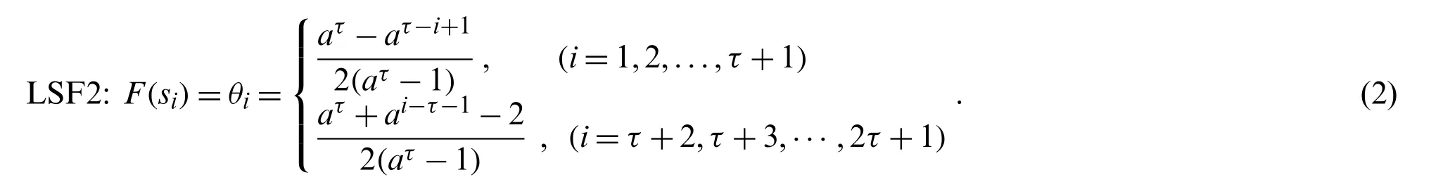
Lots of experimental studies [37] have illustrated thatagenerally lies in the interval[1.36,1.4].Moreover,aalso can be determined by a subjective approach [22].In LFS2,the absolute deviation between adjacent LTs gradually increases from the middle of the given LTs to both ends.If we take τ=3 and seta=1.36,the LTs are graphically shown in Fig.2.

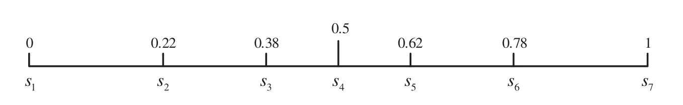
Figure 2:LSF2 (τ=3,a=1.36)

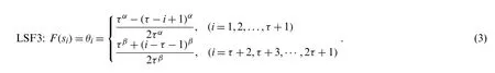
LSF3 is defined based on prospect theory’s value function and the DMs’ different sensation for the absolute deviation between adjacent linguistic subscripts.α and β (α,β ∈[0,1]) represent the curvature of the subjective value function for gain and loss,respectively [38].LSF3 reduces to LSF1 when α=β=1.The absolute deviation between adjacent LTs gradually decreases from the middle of the given LTs to both ends.If we take τ=3 and set α=β=0.8,the LTs are graphically shown in Fig.3.

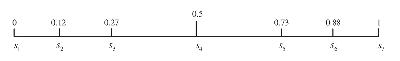
Figure 3:LSF3 (τ=3,α=β=0.8)

In order to save all of the given information and facilitate calculation,the aforesaid functions can be extended intoF*: ~S→R+,whereF*(si)=θiis a continuous and strictly monotonously increasing function.

Definition 2.[7] LetS={si|i=1,2,...,2τ +1} be a LTS.A PLTSL(p) can be defined aswheres(l)(p(l)) is the LTs(l)associated with the probabilityp(l),and #L(p) denotes the number of all different LTs inL(p).is used to normalize the PLTS.

In this paper,it is assumed that all PLTSs have already been normalized.

Definition 3.[8] LetS={si|i=1,2,...,2τ+1} be a LTS.A LHFSLHinSis defined asLH={(s(l),lh(s(l)))|s(l)∈S},wherelh(s(l))={r1,r2,...,r#lh(s(l))} is a set with #lh(s(l)) values in (0,1] and denotes the possible membership degrees of the elements(l)∈Sto the setLH.#LHdenotes the number of all different LTs inLH,and #lh(s(l)) represents the count of real numbers inlh(s(l)).

2.2 Cloud Model

Definition 4.[14] LetUbe the universe of discourse andTbe a qualitative concept inU.Ifx∈Uis a random instantiation of conceptTthat satisfiesx～N(Ex,En′2) andEn′～N(En,He2),andy∈[0,1] is the certainty degree ofxbelonging toTthat satisfiesthen the distribution ofxin the universeUis defined as a normal cloud,and (x,y) represents a cloud drop.

For simplicity,normal cloud is called as cloud hereafter.The degree of certainty ofxbelonging to conceptTis a probability distribution rather than a fixed number.Hence,∀x∈U,is a one-to-many mapping.

There are two kinds of uncertainty: randomness and fuzziness.Randomness refers to the uncertainty contained in an event that has a clear definition but do not necessarily occur.Fuzziness refers to the uncertainty contained in an event that has appeared but it is difficult to define it accurately [39].There is a practical demand to describe fuzziness and randomness inherent in LTs simultaneously.Cloud can perfectly depict the overall quantitative properties of a concept through three numerical characteristics: mathematical expectationEx,entropyEnand hyper entropyHe,whereExis the mathematical expectation of cloud drops belonging to a concept in the universe,andEnreflects the uncertainty measurement of a qualitative concept,including randomness and fuzziness.From the perspective of probability theory,Enis similar to standard variance of random variables.From the point of fuzzy set theory,Enrepresents the scope in which cloud drops are accepted by the concept,and it indicates the support set of the concept with membership degrees larger than 0.As a result,Enreflects randomness and fuzziness of a qualitative concept and their correlation,simultaneously.Herepresents the degree of uncertainty ofEn,i.e.,the second-order entropy of the entropy [15,40].A cloud can be described byEx,En,He,and denoted byC=(Ex,En,He).

Definition 5.[15] Given two cloudsC1=(Ex1,En1,He1) andC2=(Ex2,En2,He2),some operations of clouds are defined as follows:

2.3 AFSD

The AFSD is used to compare two stochastic variables.It was proposed by Leshno and Levy [41].LetX1andX2be two stochastic variables,whereG1(x) andG2(x) denote two cumulative distribution functions,respectively.Let Ω={x|G1(x)＞G2(x)},Θ={x|G2(x)＞G1(x)} andThen,AFSD is defined below:

Definition 6.[41,42] For 0＜δ＜0.5,X1dominatesX2by δ－AFSD if and only ifwhere ||G1(x)－G2(x)|| corresponds to the area betweenG1andG2,ΩG1(x)－G2(x)dxcorresponds to the area thatG1is greater thanG2,and δ denotes the degree of first-degree stochastic dominance violation allowed.

3 Heterogeneous MAGDM Problem and Comprehensive Cloud

This section describes the heterogeneous MAGDM problem and introduces the improved transformation approach between LT and cloud in detail.Particularly,we developed two novel transformation approaches from PLTS and LHFS to comprehensive clouds.

3.1 Description for Heterogeneous MAGDM Problem

A heterogeneous MAGDM problem is to find the best solution from all feasible alternatives assessed on multiple attributes by a group of DMs.The evaluation attributes in heterogeneous MAGDM can be classed into several subsets which are expressed by different kinds of forms.

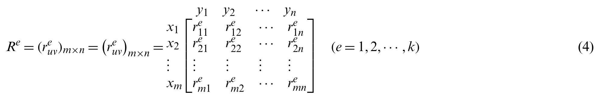
For a heterogeneous MAGDM problem,suppose that DMsde(e=1,2,···,k) have to select the optimal alternative(s) from a group of alternativesxu(u=1,2···,m) or rank these alternatives based on attributesyv(v=1,2···,n).Denote an alternative set byX={x1,x2,···,xm},an attribute set byY={y1,y2,···,yn},and a DM set byD={d1,d2,···,dk}.DenoteY1={y1,y2,···,yv1},Y2={yv1+1,yv1+2,···,yv2},Y3={yv2+1,yv2+2,···,yv3},respectively,where 1 ≤v1≤v2≤v3≤n.Namely,Yis divided into three subsetsYt(t=1,2,3),whereYt(t=1,2,3) are attribute subsets in which attribute values are expressed with LTs,PLTSs and LHFSs respectively.Yt∩Yl=Ø(t,l=1,2,3;t／=l),Yt=Y,where Ø is an empty set.DenoteM={1,2,···,m},N1={1,2,···,v1},N2={v1+1,v1+2,···,v2},N3={v2+1,v2+2,···,n},N={1,2,···,n} andK={1,2,···,k}.Denote the DM weight vector by v=(ϖ1,ϖ2,···,ϖk)T,whereis the weight of DMde,satisfying that 0 ≤≤1 (e=1,2,···,k) andDenote the attribute weight vector by w=(w1,w2,···,wn)T,wherewvis the weight of attributeyv,satisfying that 0 ≤wv≤1(v=1,2,···,n) and

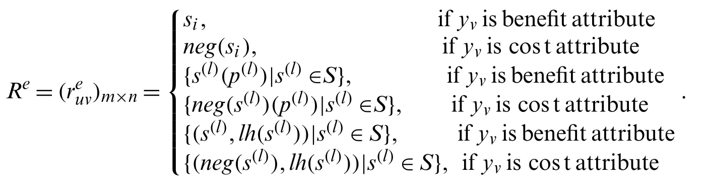
Letreuvbe the evaluation of an alternativexuon attributeyvgiven by DMde.Ifv∈N1,reuvis a LT,denoted bysi(si∈S);Ifv∈N2,reuvis a PLTS,denoted byL(p)={s(l)(p(l))|s(l)∈S};Ifv∈N3,reuvis a LHFS,denoted byLH={(s(l),lh(s(l)))|s(l)∈S}.After normalizing,the individual original normalized evaluation matrixRe=(reuv)m×ncan be obtained as

3.2 Transformation between LT and Cloud

Generally,two kinds of approaches have been proposed for transformation from LTs to clouds so far.One is based on the golden radio [44],and the other is based on the LSF [22].Wang et al.[24] introduced a parameter named overlapping degree into the transformation approach [22] to determining the degree of overlap between two adjacent clouds.With the parameter ε ∈[εmin,εmax],DMs could express their preference for the degree of overlap between two adjacent clouds.However,after processing the calculation formulae for three numerical characteristics,a problem emerges.That is,once the LSF and some related parameters are fixed in [24],andare three fixed values.It is easy to see that the values ofEniandHeiare linearly dependent onandrespectively.However,the determination of overlapping degree is entirely based on the subjective preference of DMs,which means the determination ofEniandHeiis also subjective.To overcome the above defects,two regulation parameters ς and ζ for entropy and hyper entropy are proposed in this paper.We improve the transformation approach in [24] by replacingwith ς (ζ) during the transformation process.Significantly,the determination of ς and ζ is totally objective and logical.The specific approaches to determining ς and ζ are stated in Sections 3.2.1 and 3.2.2.

LetS={si|i=1,2,···,2τ +1} be a LTS,L(p)={s(l)(p(l))|s(l)∈S} be a normalized PLTS,andLH={(s(l),lh(s(l)))|s(l)∈S} be a LHFS.denotes the evaluation of an alternativexuon attributeyv(v∈N2) given by the DMde,and #L(p)euv∈[1,2τ +1] denotes the number of all different LTs inL(p)euv.LHeuv={(s(l),lh(s(l))euv)|s(l)∈S} indicates the evaluation of an alternativexuon attributeyv(v∈N3) given by the DMde.#LHeuv∈[1,2τ +1] signifies the number of all different LTs inLHeuv.#lh(s(l))euvrepresents the count of real numbers inis a set with #lh(s(l))euvvalues in (0,1] and denotes the possible membership degrees of the elements(l)∈Sto the setLHeuv.

3.2.1 Determination of the Regulation Parameter of Entropy

EntropyEnreflects the uncertainty measurement of a qualitative concept,specifically randomness and fuzziness.From the perspective of fuzzy set theory,it represents the scope in which the cloud drops are accepted by the concept.It is common that the more elements are used in evaluations,the more hesitant the DM is.Hence,for a hesitant DM,largerEnshould to be assigned to its LTs.Therefore,the regulation parameter ofEnshould be determined according to DMs’ hesitant degree.

Definition 7.For a heterogeneous MAGDM,the average number of LTs used by DMdeat an evaluation in the form of PLTSs or LHFSs,is defined as

It is obvious that ηe∈[1,2τ+1].

Definition 8.The hesitant degree of DMdeis defined as

The determination of DM’s hesitant degree is based on the average number of LTs that DM uses at a single evaluation in the form of PLTSs or LHFSs.

A great deal of experimental research has demonstrated that regulation parameter ς generally lies in [1,2].In fact,if the hesitant degreeHDeisit means that only one LT is used by DMdeat each evaluation in the form of PLTSs or LHFSs.In this situation,DMdeis regarded as a decisive and confident person.Accordingly,it is appropriate for DMdeto take 1 as the value of ς.The more the LTs used by DMde,the bigger the value of ς is.Based on this premise,the regulation parameter ς of entropy is defined as follows:

Definition 9.Let ρ1=The regulation parameter of entropy for DMdeis defined as

where ηe∈[1,2τ+1],HDe∈Clearly,it holds that ςe∈[1,2].

In the following,an example is given to illustrate how to determine the value of ς.

Example 1.LetS={si|i=1,2,···,7} be a LTS.There are three alternativesx1,x2andx3.In order to select the optimal alternative,DMdegives evaluations forx1,x2,x3on three attributesy1,y2,y3.The evaluations fory1,y2andy3are expressed in the forms of LT,PLTS and LHFS,respectively.DMdegives an evaluation matrix as follows:

Calculate the average number of LTs used by DMdeat an evaluation in the form of PLTSs or LHFSs by Eq.(5):

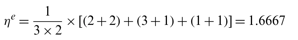
Calculate the hesitant degree of DMdeby Eq.(6):

Then,the value of ςeis calculated by Eq.(7):

ςe=log1+0.8571(0.2381+0.8571)+1=1.1470

3.2.2 Determination of the Regulation Parameter of Hyper Entropy

Hyper entropyHerepresents the degree of uncertainty ofEn,i.e.,the second-order entropy of the entropy.The largerHeis,the thicker the cloud is,and the wider the distribution of membership is.Thus,on the one hand,the information entropy as a very important concept to measure the uncertainty in evaluation information provided by DMs,the larger it is,the largerHeshould be.On the other hand,membership degree as an index to measure the degree that an element belongs to a certain concept,the lower it is,the larger the indeterminacy degree is.Furthermore,the larger indeterminacy degree in the decision matrix provided by DM,the largerHeshould to be.With the above analysis,the regulation parameter ofHeshould be determined according to indeterminacy degree and information entropy.

Definition 10.[45] The information entropy ofL(p) is defined as follows:

wherezis a constant that is set to 1.28 in this paper as [45] sets.It is easily seen thatH(L(p))∈[0,log2z·log2(2τ+1)].

Definition 11.The information entropy of DMdeis defined as follows:

wherezis a constant that is set to 1.28 in this paper as [45] sets.Obviously,He∈[0,log2z·log2(2τ+1)].

The closer the memberships for corresponding LTs are to 0,the larger indeterminacy degree DMs have for corresponding LT.

Definition 12.The indeterminacy degree ofLH={(s(l),lh(s(l)))|s(l)∈S} is defined as follows:

Clearly,it holds thatID(LH)∈[0,1).

Definition 13.The indeterminacy degree of DMdeis defined as follows:

It is easily seen thatIDe∈[0,1).

Definition 14.Let ρ2=1+log2z·log2(2τ+1).The regulation parameter of hyper entropy for DMdeis defined as

whereHe∈[0,log2z·log2(2τ+1)],IDe∈[0,1).Obviously,ζe∈[0,1).

Take τ=3 as an example.The graphical representation for the regulation parameter of hyper entropy is shown in Fig.4.

Figure 4:Graphical representation for the regulation parameter of hyper entropy (τ=3)

Example 2.Following Example 1,the value of ζecan be calculated as follows:

Calculate the information entropy of each evaluation in the form of PLTSs by Eq.(8):

H({s6(0.1),s7(0.9)})=－log21.28×(0.1×log20.1+0.9×log20.9)=0.1670,

H({s3(0.1),s4(0.2),s5(0.7)})=－log21.28×(0.1×log20.1+0.2×log20.2+0.7×log20.7)=0.4120,

H({s4(1)})=－log21.28×(1×log21)=0

Calculate the information entropy of DMdeby Eq.(9):

Calculate the indeterminacy degree of each evaluation in the form of LHFSs by Eq.(10):

Calculate the indeterminacy degree of DMdeby Eq.(11):

Then,the value of ζeis calculated by Eq.(12):

3.2.3 Specific Procedures for Transformation between LT and Cloud

Definition 15.[46] LetS={si|i=1,2,...,2τ +1} be a LTS,where τ is a positive integer.A valid universe [Xmin,Xmax] is provided by DMs.Then,a LTsi(i=1,2,...,2τ +1) can be represented by the normal cloudCi=(Exi,Eni,Hei).

Then,the specific transformation procedures are shown as follows:

(1) Calculate ς and ζ.

Determination approaches for ς and ζ are shown in Sections 3.2.1 and 3.2.2.

(2) Calculate θi.

Mapsito θiusing LSFs.

LSF2 Eq.(2) is adopted in this paper,wherea=1.36.

(3) CalculateExi.

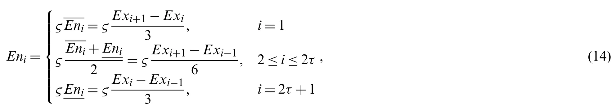
(4) CalculateEni.

Let (x,y) be a cloud drop,wherex～N(Ex,En′2).According to 3σ principle of the normal distribution,99.7% cloud drops ofCishould be located in the interval [Exi－1,Exi+1].However,since the distances betweenExiandExi－1are different from the distances betweenExiandExi+1,the entropy ofCi(i=2,3,···,2τ) are different for the right side and the left side.For simplicity,Eni(i=2,3,···,2τ) take the mean value of ςEniand.

(5) CalculateHei

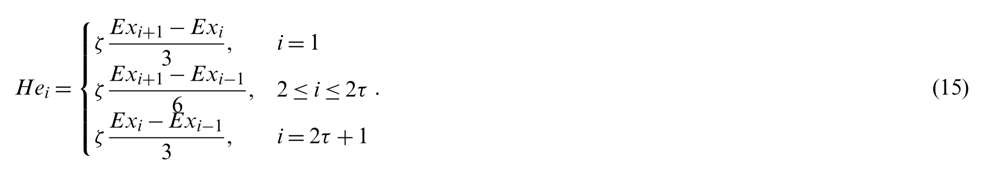
Based on the above analyses,the corresponding cloud for LTsican be generated by Algorithm 1.

Algorithm 1: Transform LT into Cloud Input: A valid universe [Xmin,Xmax],a qualitative LT si in the LTS S={si|i=1,2,...,2τ+1},and DM’s decision matrix.Output: The corresponding cloud Ci=(Exi,Eni,Hei)1.Calculate ς by Eqs.(5)–(7)2.Calculate ζ by Eqs.(8)–(12)3.Calculate θi by Eq.(1) or Eq.(2) or Eq.(3)4.Calculate Exi by Eq.(13)5.Calculate Eni by Eq.(14)6.Calculate Hei by Eq.(15)7.Return Ci=(Exi,Eni,Hei)

To illustrate the advantages of regulation parameters,an example is given below.

Example 3.Given a universe [Xmin,Xmax] and a LTSS={si|i=1,2,···,7}.For alternativesx1,x2,x3regarding three attributesy1,y2,y3,DMsd1,d2andd3give their evaluations.The evaluations fory1,y2andy3are expressed in the forms of LT,PLTS and LHFS,respectively.DMsd1,d2andd3give their evaluation matrices as follows:

Based on Eqs.(5)–(12),the regulation parameters ς and ζ for each DM are calculated as follows:

ς1=1,ζ1=0.0352,ς2=1.1470,ζ2=0.2931,ς3=1.1470,ζ3=0.6359;

Based on Eqs.(2) and (13)–(15),θi,Exi,Eni,Hei(i=1,2,···,7) for DMsd1,d2,d3are calculated and the results are shown in Tables 1–3,respectively.

Table 1:Transformation results for DM d1

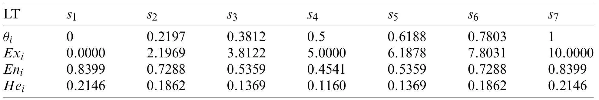
Table 2:Transformation results for DM d2

Table 3:Transformation results for DM d3

Three sets of cloud generated by DMsd1,d2,d3are graphically shown in Figs.5–7,respectively.

It can be seen from Figs.5–7 that the cloud drops distribution varies in width and thickness for different DMs.In previous studies [22,23,25–31,46],clouds for the corresponding LTS are usually the same for all DMs.However,since different DMs have different personalities,knowledge and experience,the width and thickness of clouds for the corresponding LTS should be different for different DMs.The more sure,confident and decisive the DM is for its evaluation matrix,the more concentrated and thinner the cloud distribution should be,vice versa.Unfortunately,most previous studies failed to notice this characteristic,whereas this paper sufficiently takes this characteristic into account.Although the overlap degree is considered in [24] to obtain personalized cloud sets for DMs,the determination of overlap degree depends on DMs’ subjective intuition.This defect is overcome in this paper.The regulation parameters are determined according to the evaluation matrix given by DM,which means the determination of regulation parameters is objective and logical.

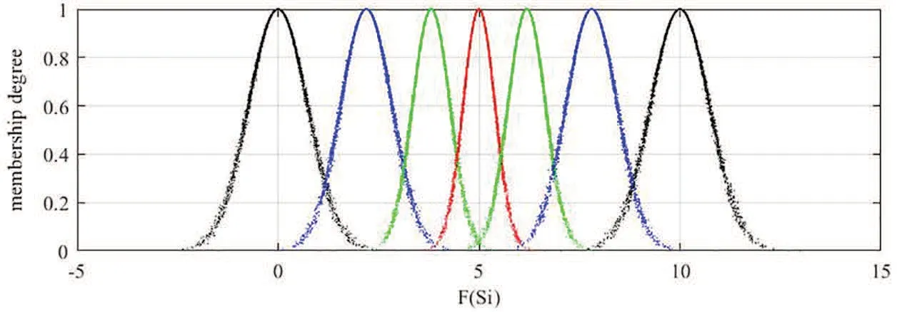
Figure 5:Clouds for the LTs used by d1

Figure 6:Clouds for the LTs used by d2

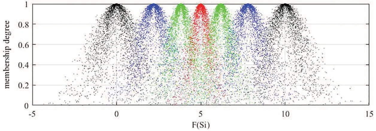
Figure 7:Clouds for the LTs used by d3

3.3 Transformation from PLTS and LHFS to Comprehensive Clouds

In this sub-section,two approaches are brought forward to transform PLTS and LHFS into comprehensive clouds,respectively.

3.3.1 Transformation from PLTS to Comprehensive Cloud

Definition 16.LetS={si|i=1,2,...,2τ+1} be a LTS.The valid universe is [Xmin,Xmax].LetL(p)={s(l)(p(l))|s(l)∈S} be a normalized PLTS.The cloudCs(l)(Exs(l),Ens(l),Hes(l)) represents LTs(l)∈S.Then,CL(p)(ExL(p),EnL(p),HeL(p)) can be defined as C-PLTS,which is characterized by three numerical characteristicsExL(p),EnL(p)andHeL(p).

Definition 17.[24] Given a cloudC=(Ex,En,He),if (x,y) is a cloud drop ofC,xsatisfiesx～N(Ex,En′2) andEn′～N(En,He2).Then,the normal curve (NC) of all cloud drops can be defined as

The specific procedures to determineExL(p),EnL(p),HeL(p)of C-PLTS are as follows:

(1) LetCs(l)be the corresponding clouds fors(l)(l=1,2,...,#L(p)),Cs(l)(p(l))beCs(l)with corresponding probabilityp(l)and χl,l+1∈[Exs(l),Exs(l+1)] be the abscissa value of intersection point between the PDFCs ofCs(l)(p(l))andCs(l+1)(p(l+1)).IfExs(l)+3Ens(l)＞Exs(l+1)－3Ens(l+1)(l∈{1,2,...,#L(p)－1}),then Eq.(16) is used to calculate the value of χl,l+1.

(2) Use Eq.(17) to calculate the area for the PDFC ofCs(l)(p(l))from lower limit to upper limit,which can be denoted byAs(l).

IfExs(l－1)+ 3Ens(l－1)≤Exs(l)－ 3Ens(l)(l∈{2,3,...,#L(p)}) (Exs(l)+ 3Ens(l)≤Exs(l+1)－3Ens(l+1)(l∈{1,2,...,#L(p)－1})),thenExs(l)－3Ens(l)(Exs(l)+3Ens(l)) is substituted for χl－1,l(χl,l+1).

(3) The modified ratio ofs(l),denoted byts(l),will be calculated by Eq.(18):

(4) According to Definition 5,three numerical characteristicsExL(p),EnL(p),HeL(p)of C-PLTS will be obtained as follows:

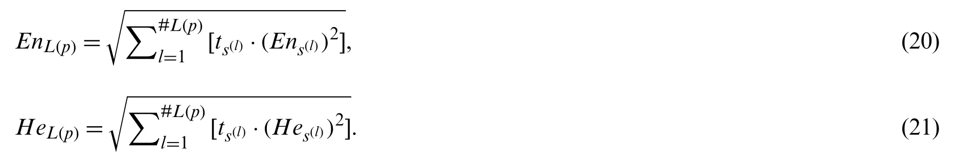
Based on the above analyses,the comprehensive cloud of PLTSL(p)={s(l)(p(l))|s(l)∈S} can be generated by Algorithm 2.

Algorithm 2: Transform PLTS into C-PLTS Input: L(p)={s(l)(p(l))|s(l)∈S} and Cs(l)(Exs(l),Ens(l),Hes(l))Output: C-PLTS CL(p)(ExL(p),EnL(p),HeL(p))1.Calculate χ by Eq.(16)2.Calculate As(l) by Eq.(17)3.Calculate ts(l) by Eq.(18)4.Calculate ExL(p) by Eq.(19)5.Calculate EnL(p) by Eq.(20)6.Calculate HeL(p) by Eq.(21)7.Return CL(p)(ExL(p),EnL(p),HeL(p))

Example 4.Given a LTSS={si|i=1,2,···,7} and a PLTSL(p)={s4(0.8),s5(0.2)},C4=(5,0.3959,0.0396) is the corresponding cloud for LTs4andC5=(6.1878,0.4672,0.0467) is the corresponding cloud for LTs5.The C-PLTSCL(p)(ExL(p),EnL(p),HeL(p)) forL(p)={s4(0.8),s5(0.2)}can be obtained as follows:

(1) Based on Eq.(16),the abscissa value of the intersection point χ is obtained:

(2) Based on Eq.(17),the area for the PDFC ofCs4(0.8)fromEx4－3En4to the intersection point and the area for the PDFC ofCs5(0.2)from the intersection point toEx5+3En5are obtained:

(3) Based on Eq.(18),the modified ratios ofs4ands5are obtained:

(4) Based on Eqs.(19)–(21),three numerical characteristics are obtained:

Finally,the C-PLTS ofL(p)={s4(0.8),s5(0.2)} isC{s4(0.8),s5(0.2)}(5.2040,0.4090,0.0409).

The PDFCs and 5000 cloud drops ofCs4(0.8)andCs5(0.2)are shown in Fig.8.The areas for the PDFCs ofCs4(0.8)andCs5(0.2)are shown in Fig.9.

Figure 8:PDFCs and 5000 cloud drops of Cs4(0.8) and Cs5(0.2)

Figure 9:Areas for the PDFCs of Cs4(0.8) and Cs5(0.2)

FromL(p)={s4(0.8),s5(0.2)},we can know that the proportions of LTss4ands5are 0.8 and 0.2,respectively.If a DM usesL(p)={s4(0.8),s5(0.2)} to evaluate an alternative,it can be assumed that the DM uses 5000 cloud drops to express his/her opinion,then he/she will place 4000 cloud drops in thes4region and 1000 cloud drops ins5region.However,it can be seen from Fig.8 that parts of the 4000 cloud drops belonging tos4region will overlap with cloud drops belonging tos5region,and parts of the 1000 cloud drops belonging tos5region will overlap with cloud drops belonging tos4region.In order to eliminate the information distortion caused by the overlapping part,this paper eliminates the overlapped cloud drops from the cloud drops originally allocated and recalculates the proportions that belong to each region.PLTS contains LTs and their corresponding probabilities.Thus the intersection point between the PDFC ofCs4(0.8)and the PDFC ofCs5(0.2)is taken as the boundary to recalculate the proportions of cloud drops distributed in the two regions,which are shown in Fig.9.From the perspective of probability,the C-PLTS is obtained.In the meanwhile,the modified ratios of LTs decrease the loss and distortion of evaluation information.

3.3.2 Transformation from LHFS to Comprehensive Cloud

Definition 18.LetS={si|i=1,2,···,2τ+1} be a LTS.The valid universe is [Xmin,Xmax].LetLH={(s(l),lh(s(l)))|s(l)∈S} be a LHFS.The cloudCs(l)(Exs(l),Ens(l),Hes(l)) represents LTs(l)∈S.Then,CLH(ExLH,EnLH,HeLH) can be defined as C-LHFS,which is characterized by three numerical characteristicsExLH,EnLHandHeLH.

The specific procedures to determineExLH,EnLH,HeLHof C-LHFS are as follows:

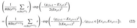
(1) LetCs(l)be the corresponding clouds fors(l)(l=1,2,...,#LH),C(s(l),lh(s(l)))beCs(l)with corresponding average value of membership degreesand χl,l+1∈[Exs(l),Exs(l+1)] be the abscissa value of intersection point between the NCs ofC(s(l),lh(s(l)))andC(s(l+1),lh(s(l+1))).IfExs(l)+3Ens(l)＞Exs(l+1)－3Ens(l+1)(l∈{1,2,...,#LH－1}),then Eq.(22) is used to calculate the value of χl,l+1.

(2) Use Eq.(23) to calculate the area for the NC ofC(s(l),lh(s(l)))from lower limit to upper limit,which can be denoted byAs(l).

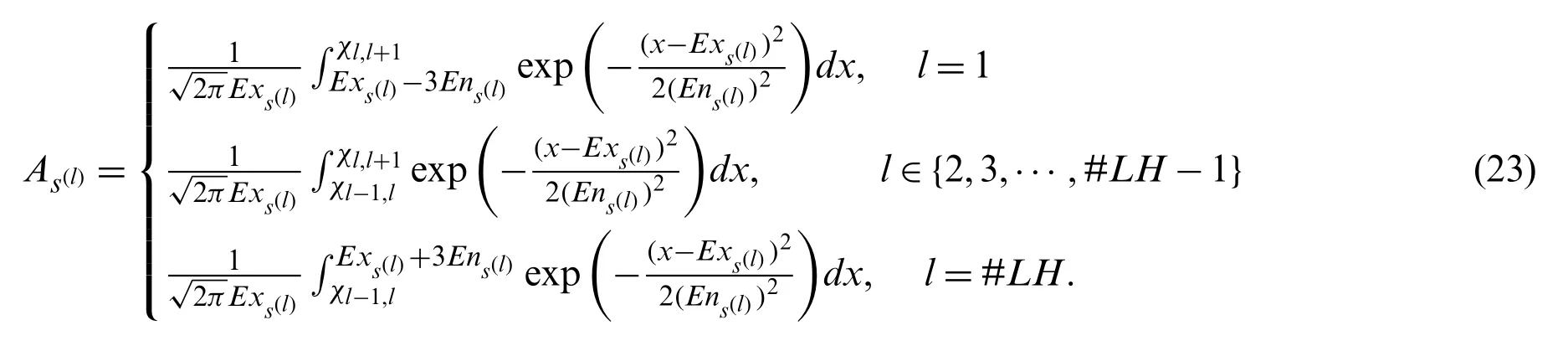
IfExs(l－1)+ 3Ens(l－1)≤Exs(l)－ 3Ens(l)(l∈{2,3,···,#LH}) (Exs(l)+ 3Ens(l)≤Exs(l+1)－3Ens(l+1)(l∈{1,2,...,#LH－1})),thenExs(l)－3Ens(l)(Exs(l)+3Ens(l)) is substituted for χl－1,l(χl,l+1).

(3) The modified ratio ofs(l),denoted byts(l),will be calculated by Eq.(24):

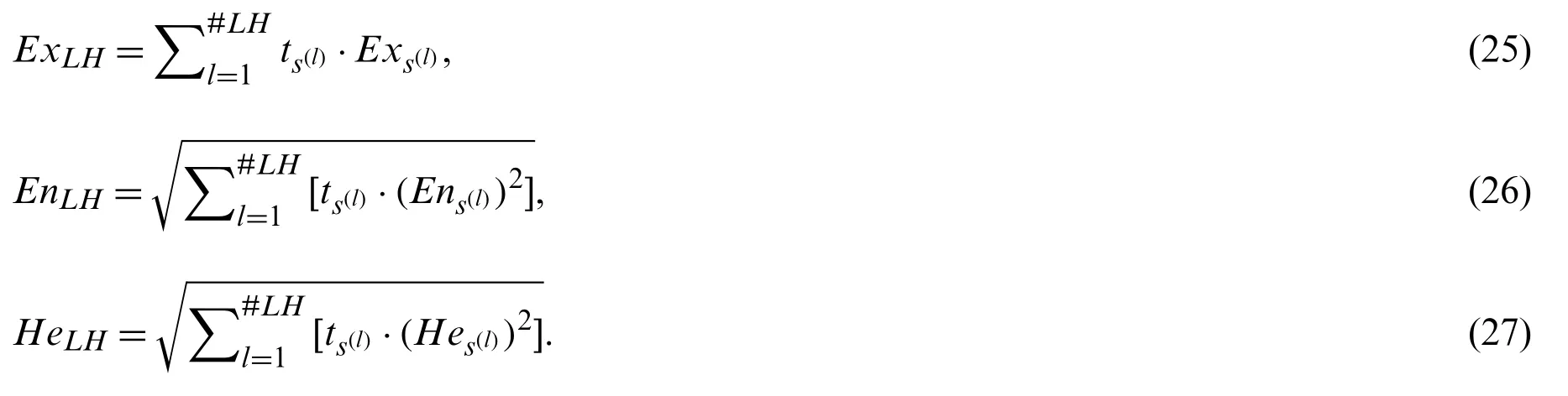
(4) According to Definition 5,three numerical characteristicsExLH,EnLH,HeLHof C-LHFS will be obtained as follows:

Based on the above analyses,the comprehensive cloud of LHFSLH={(s(l),lh(s(l)))|s(l)∈S}can be generated by Algorithm 3.

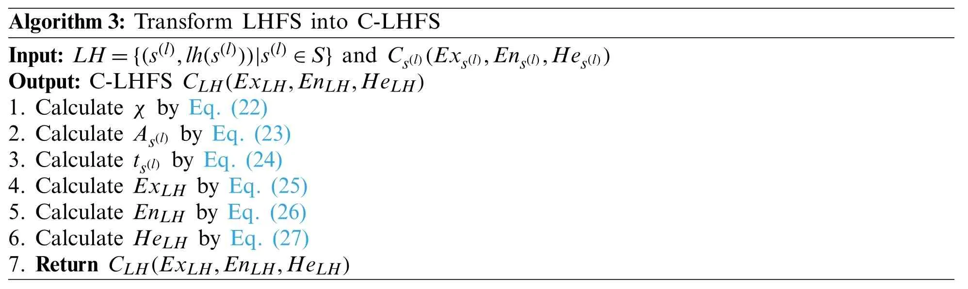
Algorithm 3: Transform LHFS into C-LHFS Input: LH={(s(l),lh(s(l)))|s(l)∈S} and Cs(l)(Exs(l),Ens(l),Hes(l))Output: C-LHFS CLH(ExLH,EnLH,HeLH)1.Calculate χ by Eq.(22)2.Calculate As(l) by Eq.(23)3.Calculate ts(l) by Eq.(24)4.Calculate ExLH by Eq.(25)5.Calculate EnLH by Eq.(26)6.Calculate HeLH by Eq.(27)7.Return CLH(ExLH,EnLH,HeLH)

Example 5.Given a LTSS={si|i=1,2,···,7} and a LHFSLH={(s5,0.6),(s6,0.9)},C5=(6.1878,0.4672,0.0467) is the corresponding cloud for the LTs5andC6=(7.8031,0.6354,0.0635)is the corresponding cloud for the LTs6.The C-LHFSCLH(ExLH,EnLH,HeLH) forLH={(s5,0.6),(s6,0.9)} can be obtained as follows:

(1) Based on Eq.(22),the abscissa value of the intersection point χ is obtained:

(2) Based on Eq.(23),the area for the NC ofC(s5,0.6)fromEx5－3En5to the intersection point and the area for the NC ofC(s6,0.9)from the intersection point toEx6+3En6are obtained:

(3) Based on Eq.(24),the modified ratios ofs5ands6are obtained:

(4) Based on Eqs.(25)–(27),three numerical characteristics are obtained:

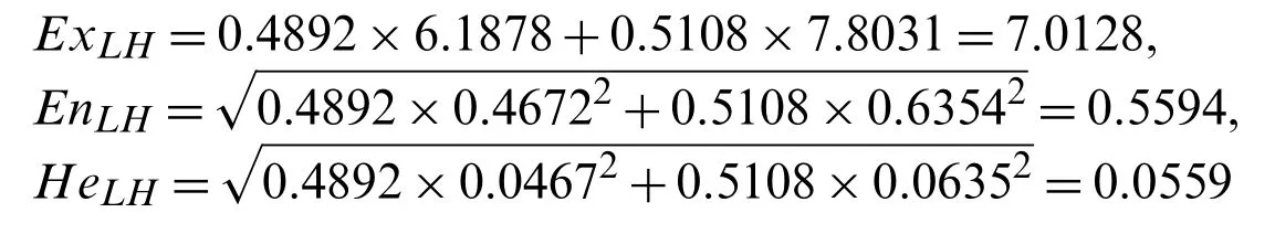
Finally,the C-LHFS ofLH={(s5,0.6),(s6,0.9)} isC{(s5,0.6),(s6,0.9)}=(7.0128,0.5594,0.0559).

The NCs and 5000 cloud drops ofC(s5,0.6)andC(s6,0.9)are shown in Fig.10.The areas for the PDFCs ofC(s5,0.6)andC(s6,0.9)are shown in Fig.11.

Figure 10:NCs and 5000 cloud drops of C(s5,0.6) and C(s6,0.9)

Figure 11:Areas for the PDFCs of C(s5,0.6) and C(s6,0.9)

FromLH={(s5,0.6),(s6,0.9)},we can know that the membership degrees of LTss5ands6are 0.6 and 0.9 respectively.If a DM usesLH={(s5,0.6),(s6,0.9)} to evaluate an alternative,it can be assumed that the DM uses 5000 cloud drops to express his/her opinion,then he/she will place 2500 cloud drops in thes5region and 2500 cloud drops ins6region.Since the membership degree of LTs5is 0.6,the maximum membership degree of cloud drops belonging tos5region should be adjusted to 0.6.For the same reason,the maximum membership degree of cloud drops belonging tos6region should be adjusted to 0.9.Similar to the process of C-PLTS,parts of the 2500 cloud drops belonging tos5region will overlap with cloud drops belonging tos6region,and parts of the 2500 cloud drops belonging tos6region will overlap with cloud drops belonging tos5region,which can be seen from Fig.10.In order to eliminate the information distortion caused by the overlapping part,this paper eliminates the overlapped cloud drops from the cloud drops originally allocated and recalculates the proportions that belong to each region.LHFS contains LTs and their corresponding membership degree.Thus the intersection point between the NC ofC(s5,0.6)and the NC ofC(s6,0.9)is taken as the boundary to recalculate the proportions of cloud drops distributed in the two regions,which are shown in Fig.11.From the perspective of membership degree,the C-LHFS is obtained.In the meanwhile,the modified ratios of LTs decrease the loss and distortion of evaluation information.

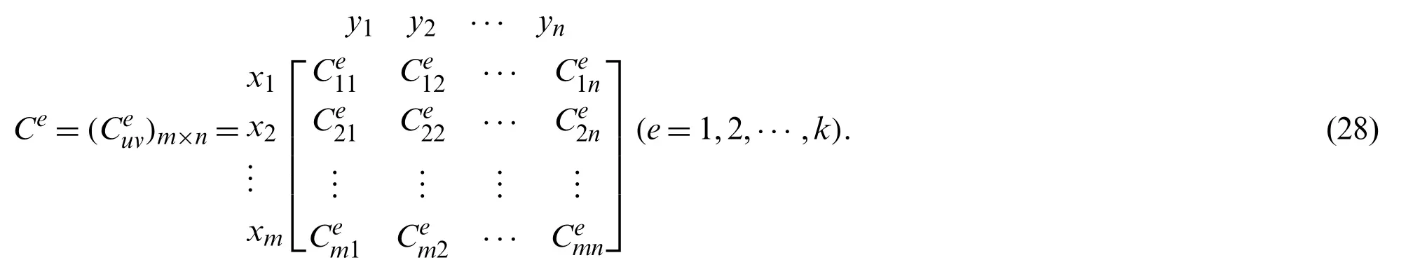
Up till now,heterogeneous MAGDM matrices in which attribute values are expressed with LTs,PLTSs and LHFSs can be transformed into homogeneous MAGDM cloud matrices.For simplicity,homogeneous MAGDM cloud matrix is called as cloud matrix hereafter.Then,the individual cloud matrixCe=(Ceuv)m×ncan be elicited as

4 Cloud-Based Heterogeneous MAGDM

In this section,some related techniques are introduced,such as the comparison approach for clouds,the determination approaches of DM weight vector and attribute weight vector.Significantly,a personalized comprehensive cloud-based method for heterogeneous MAGDM problem is proposed.

4.1 Determination of DM Weight Vector

As mentioned above,the regulation parameter ς of entropy is determined according to DMs’hesitant degree and the regulation parameter ζ of hyper entropy is determined according to DMs’indeterminacy degree and information entropy.Therefore,the larger the two parameters are,the smaller weight should be given to the DM.Assume that there are a series of regulation parameters ςe∈[1,2] of entropy and a series of regulation parameters ζe∈[0,1) of hyper entropy for DMde.Based on the regulation parameters ςeand ζe,the weight of DMdecan be calculated by

Solving Eq.(29),the DM weight vector v=(ϖ1,ϖ2,···,ϖk)Tis obtained.

Example 6.Following Example 3,ς1=1,ζ1=0.0352;ς2=1.1470,ζ2=0.2931;ς3=1.1470,ζ3=0.6359.

By Eq.(29),the DM weight vector v=(ϖ1,ϖ2,ϖ3)T=(0.4144,0.3290,0.2567)Tis obtained.

Definition 19.[22] Assume that ℵis the set of all clouds andCe(Exe,Ene,Hee)(e=1,2,···,k)is a subset of ℵ.A mapping CWAA: ℵm→ℵis defined as the cloud-weighted arithmetic averaging(CWAA) operator so that the following is true:

Based on Eqs.(29) and (30) and basic operations of clouds in Definition 5,the individual cloud matricesCe=(Ceuv)m×n(e=1,2,···,k) can be aggregated into a collective cloud matrix

Cg=(Cguv)m×nas

4.2 Pairwise Comparisons of Clouds

The evaluations from DMs have been transformed to clouds.As mentioned above,if (x,y)is a cloud drop ofC=(Ex,En,He),it is easily known thatis the PDFC ofC.LetC1=(Ex1,En1,He1) andC2=(Ex2,En2,He2) be two clouds,thengC1=are the PDFCs forC1andC2.GC1(x)andGC2(x) are the corresponding distribution functions respectively.Motivated by the comparison approach for linguistic distributions in [42],a new comparison approach for clouds is presented in the following.

4.2.1 CASD Relationship

According to the characteristics of cloud,AFSD theory is used to compare the dominance relationship between clouds with characteristicsEx,EninC=(Ex,En,He).

Definition 20.Let Ω={x|GC1(x)＞GC2(x)},Θ={x|GC2(x)＞GC1(x)},and ||GC1(x)－GC2(x)||=

IfD21＜0.5,thenC1CASDC2.It is easily seen thatD12=1－D21.Thus,ifD12＞0.5,C1CASDC2can be obtained as well.

4.2.2 CASD Degree

As mentioned above,the CASD relationship is adapted to compare two clouds.However,this relationship cannot quantify the degree for one cloud over another.To quantify the dominance degree,CASD degree is put forward.

Let μ1be the threshold for the deviation betweenEx1andEx2,μ2be the threshold for the deviation betweenEn1andEn2,and μ3be the threshold for the deviation betweenHe1andHe2.Letq12denote the CASD degree forC1overC2.IfC1CASDC2,q12can be calculated by dividing into the cases in Table 4.IfC1CASDC2,butEx1,Ex2,En1,En2,He1andHe2do not satisfy cases in Table 4,thenq12=0.5.IfC1CASDC2is not verified,thenq12=1－q21.

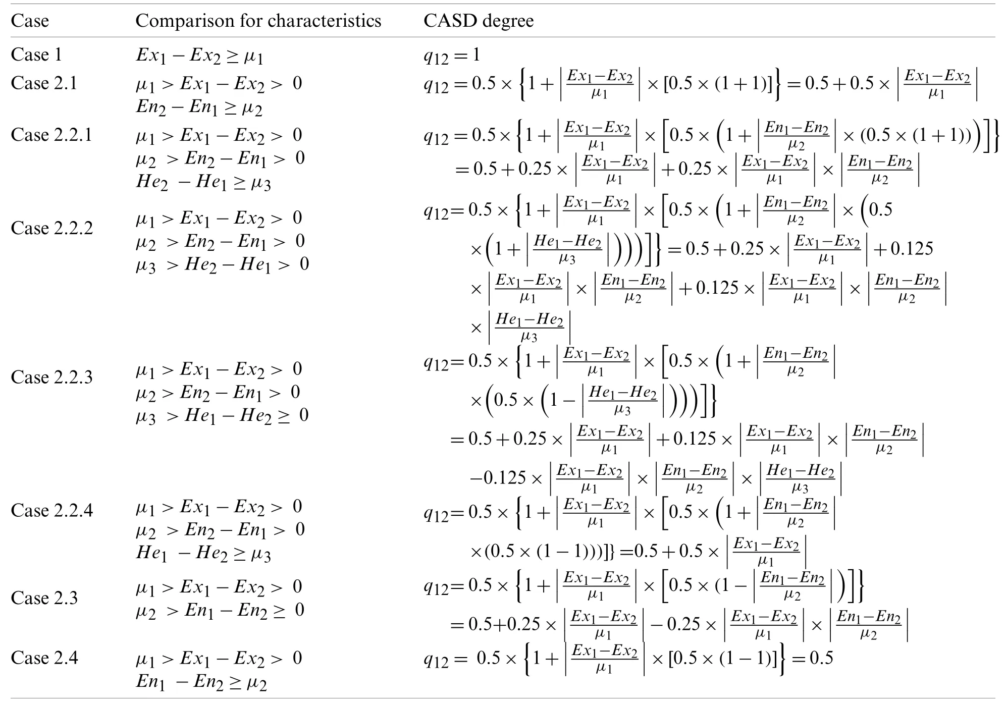
Table 4:Calculation approach of CASD degree

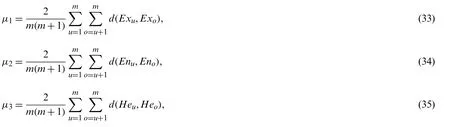
To rank the alternatives and select the optimal alternative,the comparison approach for clouds is applied to the collective cloudmatrix.Alternativesxu(u=1,2,···,m) are compared in pair on each attributeyv(v=1,2,···,n).In this paper,the values of μ1,μ2and μ3are determined as follows:

Based on the comparison approach mentioned above,the CASD degree for the alternativesxuoverxo(u,o=1,2,···,m;u／=o) with respect to attributesyvcan be calculated,denoted byquo,v.At the same time,the collective CASD degree matrixQv=(quo,v)m×mon each attributeyvis obtained:

Letquvdenote the collective overall CASD degree for alternativesxuover other alternatives with respect to attributeyv,where

Then,the collective overall CASD degree matrixQ=(quv)m×ncan be obtained

4.3 Determination of Attribute Weight Vector

As mentioned in Section 3.1,the attribute weight vector is denoted by w=(w1,w2,···,wn)T,satisfying 0 ≤wv≤1 (v=1,2,···,n) andIn this paper,three perspectives are considered to obtain the attribute weights,which are differentiation between evaluation values,relationship between attributes and the amount of information contained in evaluation values.

4.3.1 From the Perspective of Differentiation between Evaluation Values

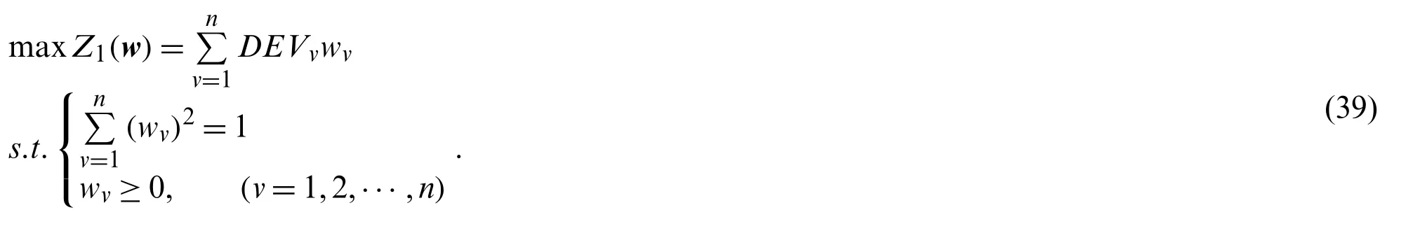
According to maximizing deviation approach [47],an attribute with a larger deviation value among alternatives should be assigned a larger weight,and vice versa.Thus,Model 1 is constructed as follows:

Model 1

4.3.2 From the Perspective of Relationship between Attributes

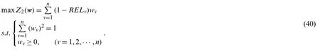
From the perspective of correlation coefficient [48],largerRELvmeans the elimination of attributeyvhas less influence on ordering and attributeyvshould be assigned a smaller weight,and vice versa.Based on correlation coefficient,Model 2 is built as follows:

Model 2

4.3.3 From the Perspective of the Amount of Information Contained in Evaluation Values

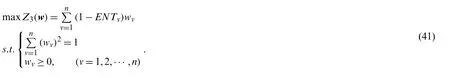
It has been mentioned in Section 3.2.2 that information entropy is an important tool to measure the uncertainty of the evaluation information.It is easily known that if the information entropy of evaluations on attributeyvis small,the difference degree contained in evaluations on attributeyvis great,which means the evaluations on attributeyvare informative and attributeyvshould be assigned a large weight,and vice versa [49].Therefore,Model 3 is constructed as follows:

Model 3

4.3.4 A Comprehensive Tri-Objective Optimization Model

Combining Eqs.(39)–(41),a comprehensive tri-objective optimization model is built as

To solve the comprehensive tri-objective optimization model,we add three balance coefficients ψ1,ψ2and ψ3into Eq.(42) and convert it into a single-objective optimization model as:

Model 4

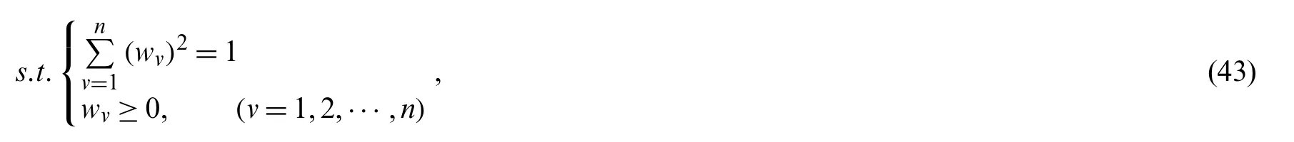
where ψ1,ψ2and ψ3are the balance coefficients,satisfying 0 ≤ψ1,ψ2,ψ3≤1 and ψ1+ψ2+ψ3=1.The values of ψ1,ψ2and ψ3could be given by DMs in advance,according to the actual situation and personal preference.

To solve Eq.(43),a Lagrange function is constructed as

where λ is a real number,denoting the Lagrange multiplier.

The global optimal solution can be derived by taking partial derivatives ofwvand λ in Eq.(44),such that

By solving Eqs.(45) and (46),the solution can be obtained

After normalizingw*v(v=1,2,···,n) in Eq.(47),we can obtain the attribute weight vector w=(w1,w2,···,wn)T,where

Model 4 enables DMs to make a tradeoff in the above three aspects.Multifaceted considerations enhance the stability of the proposed method and the setting of balance coefficients improves the flexibility of the proposed method.

4.4 Obtaining the Ranking of Alternatives

Up till now,the collective overall CASD degree matrixQ=(quv)m×nand the attribute weight vector w=(w1,w2,···,wn)Thave been obtained.Thus,the total CASD degree ofxucan be calculated as

Based on the values ofqu(u=1,2···,m),the ranking of alternatives is obtained.The largerqu,the better the alternativexu.

4.5 Decision Steps for the Personalized Comprehensive Cloud-Based Method

A personalized comprehensive cloud-based method for heterogeneous MAGDM problem is proposed in this sub-section.Particularly,the resolution procedures of the proposed method are depicted in Fig.12.

Figure 12:Resolution procedures of the proposed method

As depicted in Fig.12,the proposed method mainly includes five steps below:

Step 1.Construct the individual original normalized evaluation matrixRe=(reuv)m×nas Eq.(4).

DMs identify the feasible alternativesxu(u=1,2···,m) and determine related attributesyv(v=1,2···,n) and their evaluation forms, such as LT, PLTS, or LHFS. Each DM gives original evaluation matrixObtain the individual original normalized evaluation matrixby usingwhere

Step 2.Transform the individual original normalized evaluation matrixRe=(reuv)m×nto the individual cloud matrixCe=(Ceuv)m×nas Eq.(28).

Hesitant degreeHDe,information entropyHeand indeterminacy degreeIDefor DMdeare calculated according to the individual original evaluation matrixRe=(reuv)m×nbased on Eqs.(5),(6) and (8)–(11).Then,the regulation parameters of entropy and hyper entropy for each DM are calculated by Eqs.(7) and (12),respectively.LTs,PLTSs and LHFSs are transformed into clouds,C-PLTSs and C-LHFSs by the improved transformation approaches in Sections 3.2 and 3.3,respectively.

Step 3.Aggregate the individual cloud matricesCe=(Ceuv)m×n(e=1,2,···,k) into the collective cloud matrixCg=(Cguv)m×nas Eq.(31) with basic operations of clouds and CWAA operator.

Based on Eq.(29),DM weight vector v=(ϖ1,ϖ2,···,ϖk)Tcan be acquired according to the regulation parameters ςeand ζeof each DM.

Step 4.Transform the collective cloud matrixCg=(Cguv)m×nto the collective overall CASD degree matrixQ=(quv)m×nas Eq.(38).

Firstly,pairwise comparisons are made to judge the CASD relationships for alternativesxu(u=1,2···,m) on each attributeyvaccording to Eq.(32).Then,the thresholds forEx,EnandHeare calculated based on Eqs.(33)–(35) and the CASD degrees are calculated according to Table 4.At the same time,the collective CASD degree matricesQv=(quo,v)m×m(v=1,2,···,n)on different attributesyv(v=1,2,···,n) are obtained,as Eq.(36).Finally,calculate the collective overall CASD degreesquvfor alternativesxu(u=1,2···,m) over other alternatives on each attributeyvby Eq.(37) and generate the collective overall CASD degree matrixQ=(quv)m×n.

Step 5.Generate the ranking order of all alternativesxuaccording to the decreasing order of the total CASD degreesqu(u=1,2···,m).

Set the balance coefficients ψ1,ψ2,ψ3for Eq.(43).After obtaining the attribute weight vector w=(w1,w2,···,wn)Tby Model 4,the total CASD degrees ofxu(u=1,2···,m) can be calculated by Eq.(48).Based on the values ofqu(u=1,2···,m),the ranking of alternatives is obtained.

5 Illustrative Example

In this section,the proposed method is applied to an example of emergency medical waste disposal site selection in COVID-19.Furthermore,sensitivity analyses are conduced to demonstrate the stability and flexibility of the proposed method.

5.1 Illustration of the Proposed Method

5.1.1 Background Description

At the end of 2019,COVID-19 broke out in various provinces and cities in China.The amount of medical waste kept rising along with the number of confirmed cases.The explosive growth of medical waste occurred in many cities,and the lack of disposal capacity made the situation more serious.In such an emergency situation,medical waste disposal becomes a special battlefield in the fight against pneumonia.If these massive amounts of medical waste that may carry the virus were not disposed in a safe and timely way,it was likely to cause secondary infections and further spread of COVID-19,which may result in a series of unimaginable aftermaths.Generally,qualified medical waste disposal companies existed previously were completely at full capacity in many cities during the outbreak of COVID-19.In order to cope with the increasing amount of medical waste,many local governments adopted a series of emergency measures.One of these measures was converting other waste disposal companies,such as industrial hazardous waste disposal companies and solid waste disposal companies,to medical waste disposal sites temporarily for emergency disposal of medical waste.The selection for emergency medical waste disposal sites can be regarded as a heterogeneous MAGDM problem.

To select a suitable emergency medical waste disposal site from five alternatives{x1,x2,x3,x4,x5},a panel of four experts {d1,d2,d3,d4} were appointed to evaluate the five alternatives on five attributes: geographical location (y1),equipment (y2),process technologies (y3),disposal capacity (y4) and transport capacity (y5).The five attributes all are qualitative benefit attributes.The LTS is predefined asS={s1: very bad;s2: bad;s3: a little bad;s4: medium;s5:a little good;s6:good;s7:very good}.The evaluations for geographical location (y1) can be evaluated by LTs.PLTSs are used to evaluate equipment (y2) and process technologies (y3).LHFSs are used to evaluate disposal capacity (y4) and transport capacity (y5).The evaluations of all alternatives on the five attributes given by the four DMs are normalized and listed in Table 5.

5.1.2 Resolution Process by Using the Proposed Method of This Paper

The procedures are summarized in the following steps:

Step 1.The individual original normalized evaluation matricesRe=(reuv)5×5(e=1,2,3,4) have been obtained and presented in Table 5.

Step 2.Based on Eqs.(5)–(12),Hesitant degreeHD,information entropyH,indeterminacy degreeID,regulation parameters ς and ζ for each DM are calculated and presented in Table 6.

According to the proposed transformation approaches from LTs,PLTSs and LHFSs to clouds,C-PLTSs and C-LHFSs,the individual original normalized evaluation matricesRe=(reuv)5×5(e=1,2,3,4) have been transformed into individual cloud matricesCe=(Ceuv)5×5(e=1,2,3,4).LSF2 Eq.(2) anda=1.36 are adopted in this paper.All the individual cloud matrices are listed in Table 7.

Table 5:Individual original normalized evaluation matrices for different DMs

Table 6:Calculation results of some related indexes for DMs

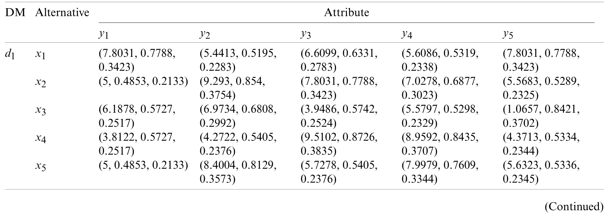
Table 7:Individual cloud matrices for different DMs

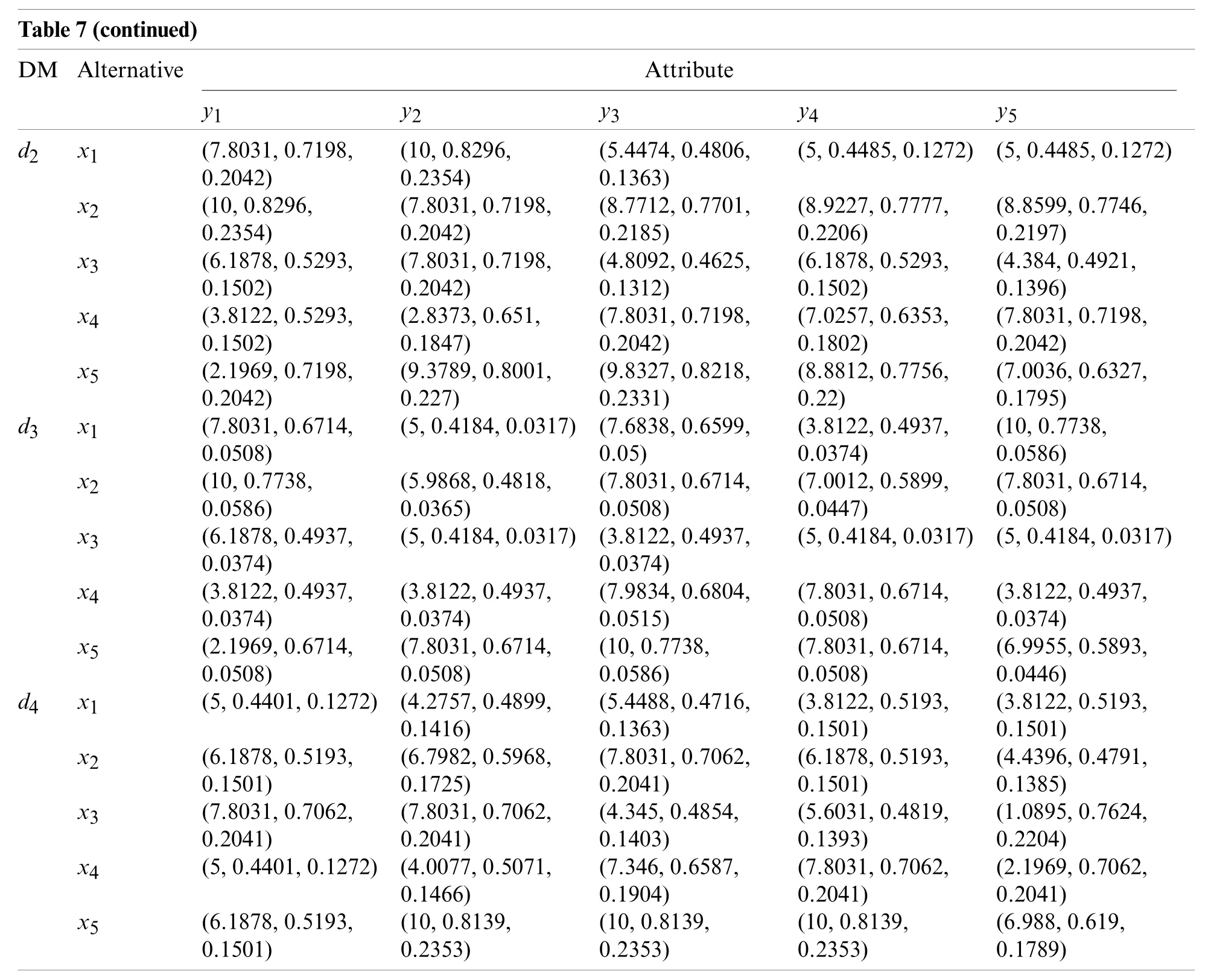
Table 7(continued)DM Alternative Attribute y1 y2 y3 y4 y5 d2 x1 (7.8031,0.7198,0.2042)(5,0.4485,0.1272) (5,0.4485,0.1272)x2 (10,0.8296,0.2354)(10,0.8296,0.2354)(5.4474,0.4806,0.1363)(8.8599,0.7746,0.2197)x3 (6.1878,0.5293,0.1502)(7.8031,0.7198,0.2042)(8.7712,0.7701,0.2185)(8.9227,0.7777,0.2206)(4.384,0.4921,0.1396)x4 (3.8122,0.5293,0.1502)(7.8031,0.7198,0.2042)(4.8092,0.4625,0.1312)(6.1878,0.5293,0.1502)(7.8031,0.7198,0.2042)x5 (2.1969,0.7198,0.2042)(2.8373,0.651,0.1847)(7.8031,0.7198,0.2042)(7.0257,0.6353,0.1802)(7.0036,0.6327,0.1795)d3 x1 (7.8031,0.6714,0.0508)(9.3789,0.8001,0.227)(9.8327,0.8218,0.2331)(8.8812,0.7756,0.22)(10,0.7738,0.0586)x2 (10,0.7738,0.0586)(5,0.4184,0.0317) (7.6838,0.6599,0.05)(3.8122,0.4937,0.0374)(7.8031,0.6714,0.0508)x3 (6.1878,0.4937,0.0374)(5.9868,0.4818,0.0365)(7.8031,0.6714,0.0508)(7.0012,0.5899,0.0447)(5,0.4184,0.0317) (5,0.4184,0.0317)x4 (3.8122,0.4937,0.0374)(5,0.4184,0.0317) (3.8122,0.4937,0.0374)(3.8122,0.4937,0.0374)x5 (2.1969,0.6714,0.0508)(3.8122,0.4937,0.0374)(7.9834,0.6804,0.0515)(7.8031,0.6714,0.0508)(6.9955,0.5893,0.0446)d4 x1 (5,0.4401,0.1272) (4.2757,0.4899,0.1416)(7.8031,0.6714,0.0508)(10,0.7738,0.0586)(7.8031,0.6714,0.0508)(3.8122,0.5193,0.1501)x2 (6.1878,0.5193,0.1501)(5.4488,0.4716,0.1363)(3.8122,0.5193,0.1501)(4.4396,0.4791,0.1385)x3 (7.8031,0.7062,0.2041)(6.7982,0.5968,0.1725)(7.8031,0.7062,0.2041)(6.1878,0.5193,0.1501)(1.0895,0.7624,0.2204)x4 (5,0.4401,0.1272) (4.0077,0.5071,0.1466)(7.8031,0.7062,0.2041)(4.345,0.4854,0.1403)(5.6031,0.4819,0.1393)(2.1969,0.7062,0.2041)x5 (6.1878,0.5193,0.1501)(7.346,0.6587,0.1904)(7.8031,0.7062,0.2041)(10,0.8139,0.2353)(10,0.8139,0.2353)(10,0.8139,0.2353)(6.988,0.619,0.1789)

Step 3.DMs’ weights are calculated by Eq.(29).With basic operations of clouds,CWAA operator,and DM weight vector v=(ϖ1,ϖ2,ϖ3,ϖ4)T=(0.1989,0.2488,0.3,0.2523)T,the collective cloud matrixCg=(Cguv)5×5is obtained and shown in Table 8.

Step 4.Compare the alternativesxu(u=1,2···,5) in pair and determinate the CASD relationships on each attributeyvby Eq.(32).The CASD degrees are calculated according to Eqs.(33)–(35) and Table 4.The collective CASD degree matricesQv=(quo,v)5×5(v=1,2···,5)are shown in Table 9.Subsequently,the collective overall CASD degrees for alternativexu(u=1,2···,5) over other alternatives on each attributeyvare calculated by Eq.(37).The collective overall CASD degree matrixQ=(quv)5×5is presented in Table 10.

Table 8:Collective cloud matrix

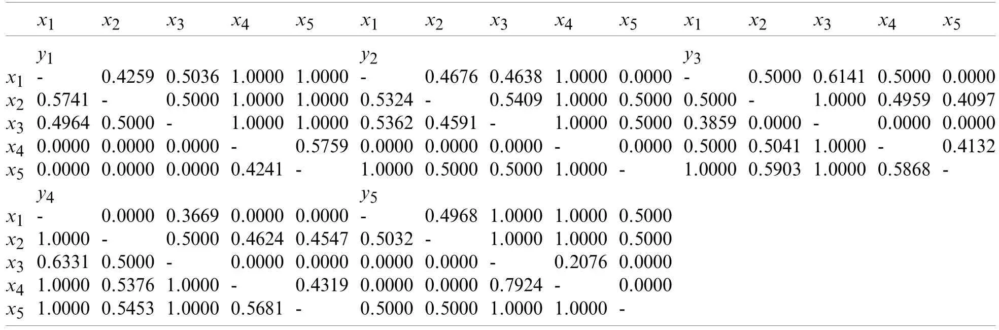
Table 9:Collective CASD degree matrices on different attributes

Table 10:Collective overall CASD degree matrix

Step5.Balance coefficientsare set for Eq.(43) in this example.By Model 4,the attribute weight vector is obtained as w=(w1,w2,w3,w4,w5)T=(0.2368,0.1886,0.1664,0.2036,0.2046)T.

With the obtained attribute weight vector,the total CASD degrees ofqu(u=1,2···,5) are calculated by Eq.(48) and the results are listed as follows:

q1=0.5036,q2=0.68,q3=0.3794,q4=0.3263,q5=0.6107

Thus,the ranking order isx2≻x5≻x1≻x3≻x4andx2is the optimal alternative.

5.2 Sensitivity Analyses

LSFs are strictly monotonously increasing with respect to the subscripti.In linguistic evaluation scales,the absolute deviation of semantics between any two adjacent LTs may increase,decrease or remain unchanged with increasing linguistic subscripts.DMs can choose different LSFs according to the actual situation and personal preference.In Eq.(43),ψ1,ψ2,ψ3are considered as the balance coefficients for each perspective of attribute weights obtaining,satisfying 0 ≤ψ1,ψ2,ψ3≤1 and ψ1+ψ2+ψ3=1.The values of ψ1,ψ2,ψ3are given by DMs in advance.This sub-section takes different LSFs and different balance coefficients to solve the above example.The corresponding decision results are listed in Table 11 and shown in Fig.13.The average differences of total CASD degrees between two adjacent alternatives in ranking results are shown in Fig.14.

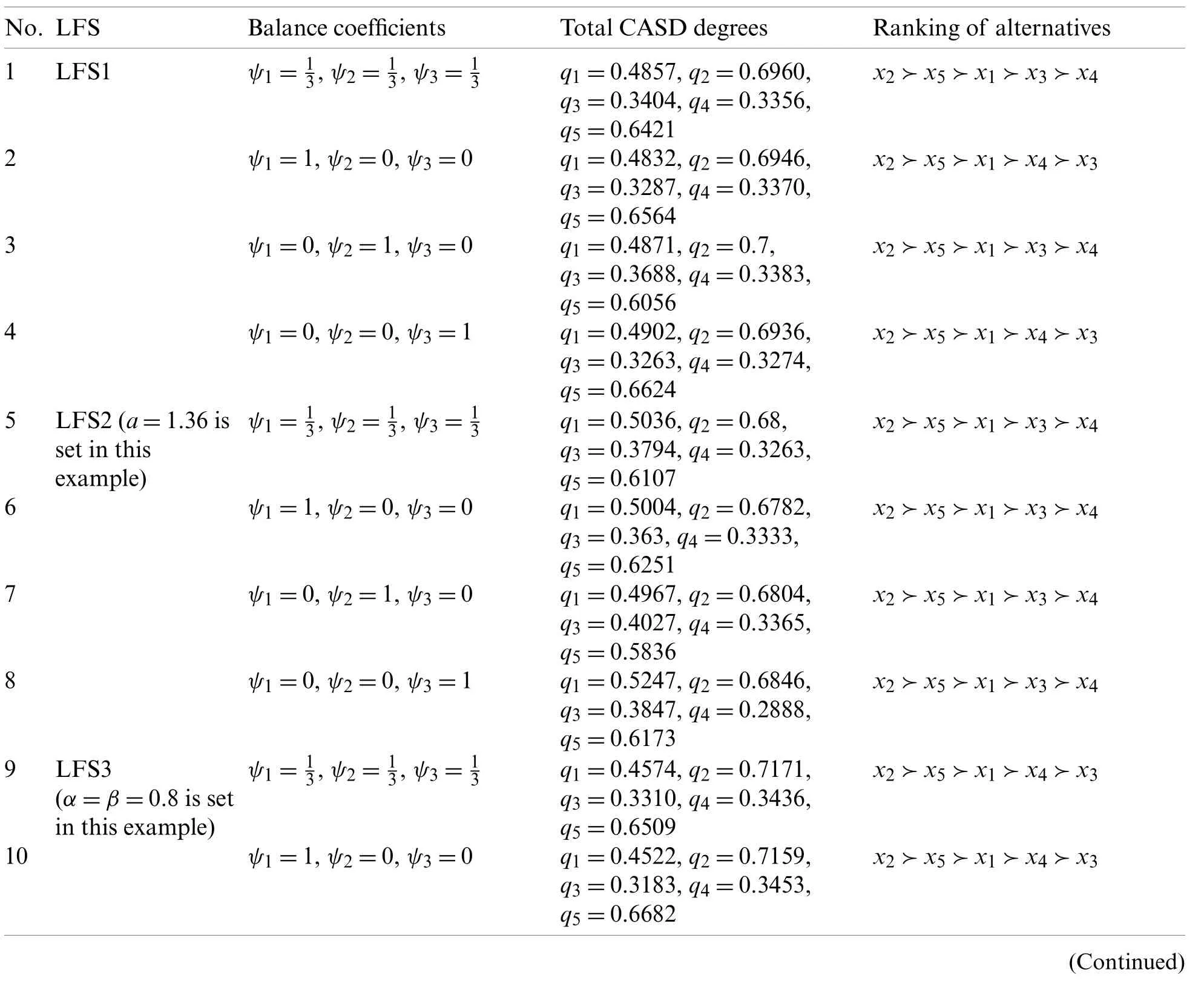
Table 11:Decision results for different LSFs and balance coefficients

Table 11(continued)No.LFS Balance coefficients Total CASD degrees Ranking of alternatives 11 ψ1=0,ψ2=1,ψ3=0 q1=0.4694,q2=0.7202,q3=0.3637,q4=0.3395,q5=0.6071 12 ψ1=0,ψ2=0,ψ3=1 q1=0.4522,q2=0.7155,q3=0.3131,q4=0.3455,q5=0.6737 x2 ≻x5 ≻x1 ≻x3 ≻x4 x2 ≻x5 ≻x1 ≻x4 ≻x3

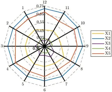
Figure 13:Demonstration of ranking results

Figure 14:Average differences of total CASD degrees

As can be seen from Table 11 and Fig.13,the ranking order of alternatives isx2≻x5≻x1≻x3≻x4orx2≻x5≻x1≻x4≻x3.Besides,it is easy to discover from Table 11 that the top three alternatives are alwaysx2,x5andx1,which indicates that the alteration of LSFs and balance coefficients has only little impact on the ranking order of the alternatives.Therefore,the proposed method has high stability in determining the optimal alternative.

Furthermore,the proposed method can handle various decision situations and meet different DMs’ preferences by taking different LSFs and balance coefficients.Thus,the flexibility of the proposed method can be reflected by the acquired ranking results derived by various selections of LSFs and balance coefficients.

6 Comparison Analyses and Discussion

To justify the advantages of our proposal,comparison analyses with methods based on cloud and other classical MAGDM methods are conducted.Besides,a summary of transformation approaches with different evaluation forms is presented.

6.1 Comparison with Methods Based on Cloud

Peng et al.[23] proposed a new method based on cloud to handle MAGDM problems with PLTSs.Hu [32] proposed two methods based on comprehensive cloud aggregation operator to solve MAGDM problems with LHFSs.This paper proposes a novel method based on cloud for heterogeneous MAGDM,which could handle MAGDM problems with LT,PLTS,LHFS or one of them.Obviously,the aforesaid methods all are based on cloud.The proposed method could handle MAGDM problems in [23,32],while Peng et al.’s method [23] and Hu’s methods [32] could not solve the problem of this paper.Thus,the proposed method has wider applicability.Except for wider applicability,other important distinguishing factors and superiorities of the proposed method are stated as follows:

(1) The cloud in [23] contains five characteristics,yet the values of left and right entropy are averaged into one in this paper,which greatly reduce the complexity of the following calculation.The transformation from LTs to clouds in [32] is based on the golden radio,while it is based on LSFs in this paper.The selection for LSFs and its related parameters makes the transformation more flexible and practical.In addition,this paper proposes regulation parameters for entropy and hyper entropy.DMs’ personalities can be reflected with the incorporation of regulation parameters in the transformation from LTs to clouds.Moreover,the modified ratios of LTs decrease the loss and distortion of evaluation information in the transformation from PLTSs (LHFSs) to C-PLTSs (C-LHFSs).

(2) The method in [23] determines the attribute weights only via maximizing deviation,while three perspectives are considered to obtain the attribute weights in this paper.Besides,the setting of balance coefficients enhances the flexibility of the proposed method.Moreover,three steps are needed to obtain attribute weights in [23],including determining the individual weights of criteria,determining the weights associated with groups (equivalent to DMs in this paper) and calculating the overall weights of attributes.By contrast,only one step is needed to obtain attribute weights by the proposed method,which reduces the complexity of the calculation greatly.

(3) The proposed approach to determining DMs’ weights is superior to [32].Hu [32] and this paper both consider the number of LTs and corresponding indeterminacy degree in LHFS.However,if all the DMs only use one LT with different memberships in all LHFSs,the determination approach of DMs’ weights in [32] becomes invalid.For example,d1andd2give their evaluation matrices as follows:

It can be seen thatd1andd2does not have the same confidence for their own evaluation matrices,but they will be assigned the same weight in [32].However,d1andd2will be assigned different weights in this paper for their different membership for LTs.Obviously,the determination approach of DMs’ weights in this paper is more reasonable.

(4) The ranking of alternatives is based on the expected score values of clouds in [32].The expected score values of clouds sometimes are unstable and may lead to inaccurate decision results.By contrast,the ranking of alternatives is based on the total CASD degree in this paper.Obviously,the ranking approach of this paper is more stable.

6.2 Comparison with Other Classical MAGDM Methods

Lin et al.[50] put forward two novel TOPSIS-ScoreC-PLTS and VIKOR-ScoreC-PLTS methods to handle MAGDM problems with PLTSs.This paper proposes a personalized comprehensive cloud-based method for heterogeneous MAGDM,which could handle MAGDM problems with LT,PLTS,LHFS or one of them.To justify the advantages of our proposal,comparison analyses with Lin et al.’s method [50] are conducted as follows:

(1) Solve the adapted example of this paper by the methods in [50]

Since Lin et al.’s method just cloud handle the MAGDM problems with PLTSs,we only retain the evaluations ony1,y2andy3in the site selection example of emergency medical waste disposal and replace Eq.(12) by ζe=logρ2(He+1).The adapted problem is dealt with the TOPSISScoreC-PLTS method in [50],the VIKOR-ScoreC-PLTS method in [50] and the proposed method,respectively.The ranking results are displayed in Table 12.

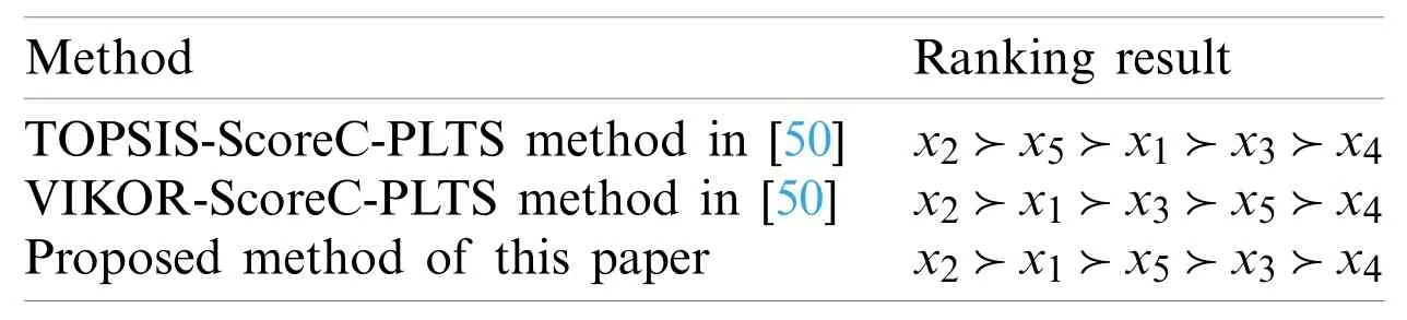
Table 12:Ranking results with different methods

It is easy to find thatx2is always the optimal alternative andx4is always the worst alternative,which shows the effectiveness of the proposed method.

(2) Solve the example in [50] by the proposed method of this paper

The proposed method could handle MAGDM problems with LT,PLTS,LHFS or one of them.As a result,the proposed method could settle the example in [50] directly and the calculation results are as follows:

DM weight vector: v=(ϖ1,ϖ2,ϖ3,ϖ4)T=(0.2415,0.2399,0.2545,0.2641)T.

Attribute weight vector: w=(w1,w2,w3,w4,w5)T=(0.2071,0.2331,0.1871,0.2205,0.1523)T.

The total CASD degrees:q1=0.6808,q2=0.4606,q3=0.3932,q4=0.4654.

Therefore,the final ranking order isx1≻x4≻x2≻x3andx1is the optimal alternative.

The ranking order by method in [50] isx1≻x2≻x3≻x4andx1≻x3≻x2≻x4.No matter by method in [50] or the proposed method,x1is the best alternative.However,the ranking of the rest alternatives differs greatly.Obviously,the most remarkable difference is the ranking order ofx4.After analysis,it is easily found that equal weights are given to each DM directly in [50],while higher weights are given to DMs with more informative evaluations in this paper.DMsd3andd4are given higher weights for their informative evaluations and they give overwhelming evaluations tox4ony1.Thus,the ranking ofx4improves a lot by the proposed method.It is clear that the proposed method of this paper is more objective and practical.

6.3 Comparison with Other Transformation Approaches

Previous studies [22–27,30–34] have proposed a lot of transformation approaches from LT and its’ extended forms to cloud and comprehensive clouds.A specific summary is shown in Table 13.

Table 13:A summary of transformation approaches with different evaluation forms

In summary,we find that most existing studies can only process LTs,or LTs with probability,or LTs with membership or LTs with interval concept.However,this paper provides the transformation approaches for LTs,LTs with probability and LTs with membership,simultaneously.Moreover,there are few studies that take DMs’ personalities into account during the transformation process.Although Wang et al.[24] introduced overlap parameter into the transformation process to reflect the DMs’ personality,the determination of overlap parameter is a little subjective.This paper proposes regulation parameters for entropy and hyper entropy and further incorporates them into the transformation process from LTs to clouds to reflect the different personalities of DMs.It is worth emphasizing that the determination of regulation parameters is totally objective.Apparently,the proposed transformation approaches of this paper are more applicable and effective.

7 Conclusion

This paper develops a personalized comprehensive cloud-based method for heterogeneous MAGDM,in which the evaluations of alternatives on attributes are represented as LTs,PLTSs and LHFSs.The validity of the proposed method is demonstrated with a site selection example of emergency medical waste disposal in COVID-19.The effectiveness,stability,flexibility and superiorities of the proposed method are proven by sensitivity and comparison analyses,respectively.Compared with the existing methods,the proposed method of this paper has the following prominent superiorities:

(1) With the proposed regulation parameters,the width and thickness of clouds for the corresponding LTS are different for different DMs,which makes the DMs’ personalities can be reflected in clouds.Besides,a novel approach to obtaining DM weight vector is constructed based on the proposed regulation parameters.

(2) The new transformation approaches from PLTS and LHFS to C-PLTS and C-LHFS decrease the loss and distortion of evaluation information.

(3) CASD relationship and CASD degree are initiated in this paper to compare clouds.With CASD relationship and CASD degree,alternatives in the form of clouds can be ranked and the ranking results are stable and effective.This innovation provides new perspective for pairwise comparisons of clouds.

(4) The comprehensive tri-objective programing constructed in this paper enables DMs to make a tradeoff among three different aspects.Multifaceted considerations enhance the stability of the proposed method and the setting of balance coefficients improves the flexibility of the proposed method.

Although an example of emergency medical waste disposal site selection in COVID-19 is illustrated to the effectiveness of the proposed method,and it is expected to be applied to more real-life decision-making problems,such as investment selection,supply chain management,and so on.More effective transformation approaches for other evaluation forms,especially LTs with interval concept are waiting for us to come up with and apply them to heterogeneous MAGDM problems.Additionally,how to extend some classical decision-making methods to heterogeneous MAGDM based on cloud is also very interesting and deserves to be studied in the future.

Funding Statement: This research was supported by the National Natural Science Foundation of China (Nos.62141302,11861034 and 71964014),the Humanities Social Science Programming Project of Ministry of Education of China (No.20YJA630059),the Natural Science Foundation of Jiangxi Province of China (No.20212BAB201011),and the Postgraduate Innovation Fund Project of Jiangxi Province (No.YC2020-S290).

Conflicts of Interest: The authors declare that they have no conflicts of interest to report regarding the present study.