Behavior of wood basic density according to environmental variables

Gabriel Marcos Vieira Oliveira ·José Márcio de Mello ·Carlos Rogério de Mello ·José Roberto Soares Scolforo ·Eder Pereira Miguel ·Thiago Campos Monteiro

Abstract The relationships between climate conditions and wood density in tropical forests are still poorly understood. To quantify spatial dependence of wood density in the state of Minas Gerais (MG, Brazil), map spatial distribution of density, and correlate density with climate variables, we extracted data from the Forest Inventory of Minas Gerais for 1988 trees scaled throughout the territory and measured wood density of discs removed from the trees. Environmental variables were extracted from the database of the Ecological-Economic Zoning of Minas Gerais. For spatial analysis, tree densities were measured at 44 georeferenced sampling points. The data were subjected to exploratory analysis, variography, cross-validation, model selection, and ordinary kriging. The relationships between wood density and environmental variables were calculated using dispersion matrices, linear correlation, and regression. Wood density proved to be highly spatially dependent, reaching a correlation of 96%, and was highly continuous over a distance of 228 km. The distribution of wood density followed a continuous gradient of 514-659 kg m-3, enabling correlation with environment variables. Density was correlated with mean annual precipitation (- 0.57), temperature (0.63), and evapotranspiration (0.83). Geostatistical methods proved useful in predicting wood density in native tropical forests with different climate conditions. Our results confirmed the sensitivity of wood density to climate change, which could affect future carbon stock in forests.

Keywords Biomass·Climate variables·Geostatistics·Hardwood·Forest inventory·Minas Gerais

Introduction

Wood density is an important variable for accurately quantifying woody biomass (Woodcock 2000; Vieira et al. 2008), carbon stocks (Sanquetta et al. 2016; Colmanetti et al. 2018), and successional stages in the forest (Plourde et al. 2015; Crouzeilles et al. 2017). Its importance arises from its easy, quick, and non-destructive determination (Gao et al. 2017; Olale et al. 2019). In addition, wood density varies greatly in correlation with other wood properties, and its values depend on the genetic material of the tree, environmental variables, and interactions between these factors (Zobel and Jett 1995; Longui et al. 2017; Barbosa et al. 2019). Thus, knowledge on wood density is essential for comprehending the responses of native forests to the diversity of environmental conditions (Cermák et al. 2015; Gomes et al. 2019).

The methods for estimating density and understanding its relations are not only dendrometric but also spatial and environmental. Some authors report important environmental influences that can affect patterns of wood density; however, their studies generally have been limited to species in commercial plantations (Antonova and Stasova 1997; Bergès et al. 2008; Kantavichai et al. 2010; Downes et al. 2014; Filipescu et al. 2014; Martinez-Antunez et al. 2015; Barbosa et al. 2019; Freitas et al. 2019; Costa et al. 2020a). Studies of the effect of the environment on wood density of tropical native species are few, inconclusive, restricted to a single species or a small groups of species (Baker et al. 2004; Muller-Landau 2004; Chave et al. 2006; Oliveira et al. 2012; David et al. 2017; Kenzo et al. 2017).

In general, variation in wood density in natural environments has been assumed to be entirely attributable to variation in species composition (Nogueira et al. 2007). However, Chave et al. (2006) reported that variation in certain environmental factors leads to spatial patterns in wood density. Likewise, Oliveira et al. (2012) reported a consistent theoretical connection between wood density and environmental characteristics in which environments that are favorable for the development of species support a higher concentration of trees with lower wood density, with the converse for unfavorable environments. Nonetheless, Kenzo et al. (2017) stated that wood density did not vary between a dry evergreen forest and a dry deciduous forest in central Cambodia.

Temperature and precipitation also affect the structure of trees in native forests, and leaf area can be used as an indicator of species sensitivity to climate change (Bohora Schlickmann et al. 2020). Not unexpectedly, periods of prolonged drought result in increased mortality rates of larger trees and, thus, a decline in aboveground carbon (Meira-Junior et al. 2020). Although forest production efficiency rises with precipitation and temperature (Collalti et al. 2020), little information is available on the effect of environmental variables on wood density and, consequently, on carbon stock, mainly in areas that cover different forest biomes.

Research on the effect of environment on the wood density of tropical native species can be aided by geostatistics, a consolidated set of robust statistical methods to analyze data that vary in space and thus detect spatial-dependence structures in forest areas (Mello et al. 2005, 2009; Guedes et al. 2012; Bardi et al. 2016; Silveira et al. 2018, 2019; Costa et al. 2020b). For example, data on wood density from a forest inventory of native areas and data on climate zoning can be analyzed together using geostatistical techniques. The results can also be used to describe already published patterns. Here, we thus aimed to identify the assumed spatial dependence structure of wood density in native forests in the state of Minas Gerais (MG, Brazil), generate a distribution map of this variable, and reveal possible correlations with environmental variables.

Material and methods

Wood density

Our density data were obtained from the Forest Inventory of Minas Gerais (Scolforo et al. 2008). We analyzed data from 1988 trees scaled throughout the state of Minas Gerais (Brazil). Sampled trees had diameters greater than 5 cm and were distributed in eight classes each for diameter and height. The trees were georeferenced, sampled in 24 different hydrographic basins and sub-basins, and represented all forest physiognomies within the state. The number of scaled trees was proportional to the relative density of the species obtained in the Forest Inventory. This criterion was applied to the four species with the highest relative density, and the others were grouped and computed as miscellaneous, as detailed by Oliveira (2014).

The scaling procedure was performed in accordance with theHubermethod (Scolforo et al. 2008; Oliveira et al. 2014). After scaling, a chainsaw was used to remove wood discs with 30 mm thickness from heights corresponding to 0, 25, 50, 75, and 100% of the commercial height of the stem. The tallest disc of the trunk had a diameter of 30 mm. Two opposing wedges that included the pith were removed from each of the five wooden discs. The wood basic density of each wedge was then determined according to NBR 11941 (ABNT 2003) as in Eq. 1:

whereBdis wood basic density (g cm-3);m3is mass (g) of oven-dried sample (105 °C ± 2 °C);m2= container mass with water and immersed disc (g); andm1= container with water (g).

The basic density of each disc was obtained based on the mean of the two wedges, and the arithmetic mean of the density of the five discs was used to generate the general basic density of the tree bole, in accordance with the methodology recommended by Vismara (2009).

Environmental variables

Environmental data were obtained from the climate data recorded at 39 climatological stations of the Ecological-Economic Zoning (EEZ) of Minas Gerais. Precipitation (mm a-1), temperature (°C), and potential evapotranspiration (mm a-1) were obtained from climatological normals for the period 1961 to 1990. Official data of the Brazilian Government available at the time of the tree collection (between 2004 and 2007) and a methodology similar to that adopted by Nelson et al. (2020) were employed. Climate maps were prepared for the entire state by means of spatial interpolation on ArcGIS Desktop v.10 (ESRI 2010), using cokriging supported by elevation, longitude, and latitude (Oliveira and Carvalho 2008).

Spatial analysis

We estimated mean wood density of trees sampled at 44 sampling sites, each site serving as a sample unit in spatial analysis. The number of trees sampled at each sampling site ranged from 17 to 126. The geographical coordinates defining each of our 44 sampling sites corresponded to the average of the coordinates recorded for each sampled tree. The Albers Projected Coordinate System (metric) was adopted under the South American Datum (1969).

The data were subjected to exploratory analysis by dispersion graphs of the variable in relation to longitude (X), latitude (Y), and histograms of frequency to verify possibly divergent observations, normality, and/or bias that could interfere with the analysis.

The spatial dependence structure of the variable was established according to the experimental semivariogram from the semivariance estimator^γ(h) (Eq. 2) in the distance function (Landim 2006; Burrough et al. 2015).

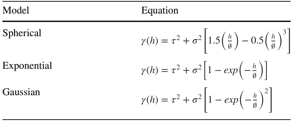
To analyze model spatial continuity, we tested three theoretical models, viz. spherical, exponential, and Gaussian, as described by others (Journel and Huijbregts 1978; Isaaks and Srivastava 1989; Burrough et al. 2015).The models were adjusted by the ordinary least squares (OLS) and weighted least squares (WLS) methods (Table 1).

Table 1 Authorized isotropic models tested: spherical, exponential, and Gaussian, and their respective equations

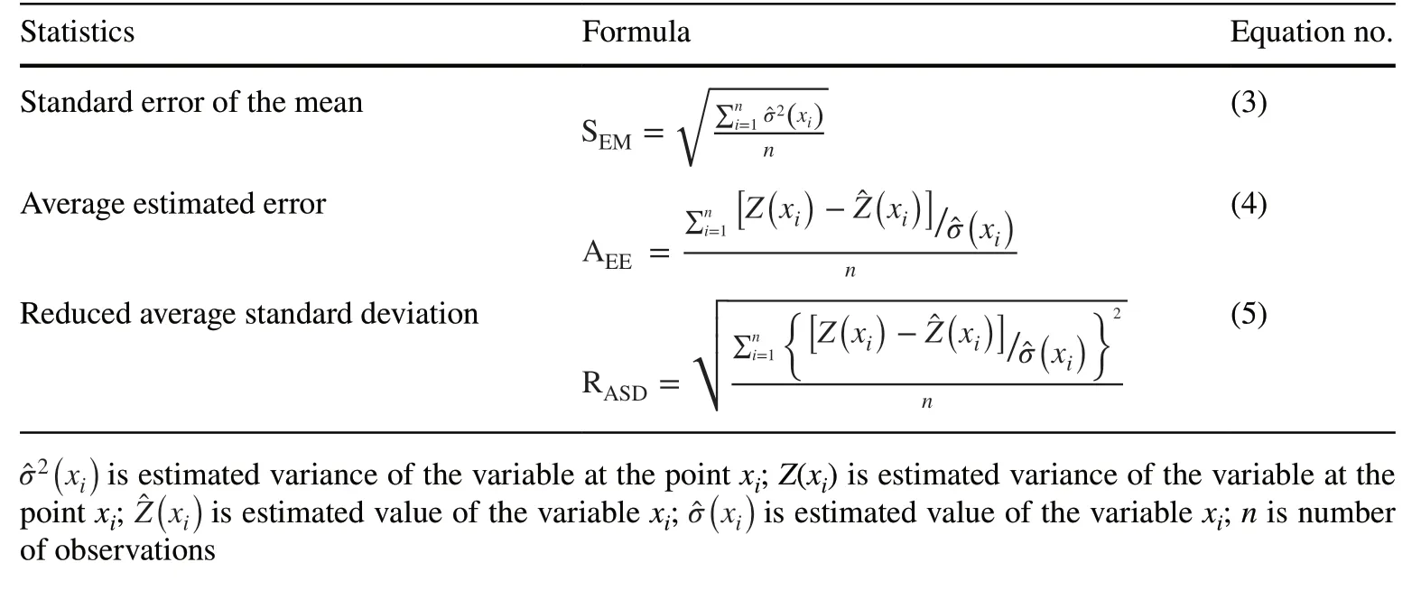
Table 2 Cross-validation error statistics: mean standard error, average estimated error, and reduced average standard deviation, and their respective equations

To select the most suitable model and the adjustment method that best described the spatial continuity of wood density, we calculated error statistics as standard error of the mean (SEM) (Eq. 3), mean reduced error (MRE) (Eq. 4), and reduced average standard deviation (RASD) (Eq. 5) obtained from the cross-validation procedure (Table 2).

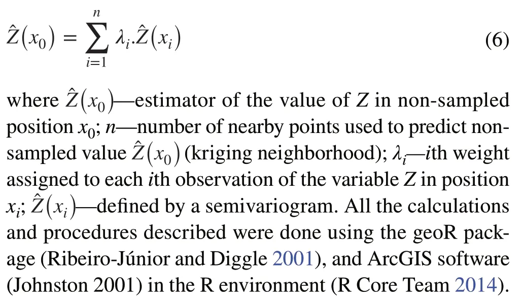
The model with the best adjustment indices (indicated by lower SEM, lower MRE, and RASD closer to one unit) was used for the spatialization of wood density for the entire state by ordinary kriging, whose estimator is given by Eq. (6) (Cellmer 2014; Chilès and Desassis 2018).

Relation between wood density and environmental factors

Relationships between wood density spatialized by kriging and the rasters of environmental factors (precipitation, temperature, and potential evapotranspiration) were compared based on the zoning of each of these variables in the 40 subbasins of Minas Gerais.

Analysis of the relationships between the variables (precipitation, temperature, and potential evapotranspiration) was verified using a dispersion matrix, Pearson linear correlation, and simple linear regression. These regression models were adjusted by the OLS method (Charnet et al. 1999).

Results

Data analyses

Considering the semivariogram (Fig. 1), spatial correlation of the variable of interest was detected after bias was removed. Semivariance continuously increased as distance increased, followed by a stabilization tendency (Mello et al. 2005; Pelissari et al. 2017). Therefore, wood density was not randomly distributed. The results also revealed an adjustment that intercepted near zero on both axes and had an asymptotic tendency of semivariance between 1000 and 1500 (kg m-3)2at distances of 200 - 300 km from the observations.

Fig. 1 Experimental semivariogram of wood density adjusted by the exponential model

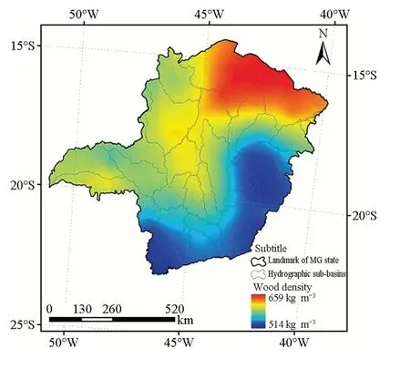
Fig. 2 Spatial distribution of the mean wood density in the state of Minas Gerais, Brazil

For the experimental semivariogram adjustment, the cross-validation error statistics proved the exponential model adjusted by the OLS method to be the most appropriate one to represent the spatial dependence structure, as it proved to have the best statistics (Table 3).

Table 3 Adjusted parameters of the exponential model and crossvalidation statistics

Based on the adjusted model after performance testing, an ordinary kriging procedure of wood density was executed for the state of Minas Gerais to compile a map that described the spatial distribution of the variable (Fig. 2). The highest wood density values of ～ 659 kg m-3were recorded in the northern region of Minas Gerais. The lowest wood densities were recorded in the southern and eastern regions of the state at values of ～ 514 kg m-3. Intermediate density values (yellow color) were recorded in the central region.

Relation between wood density and climate conditions

Quantitative analysis showed that the relationships modeled were represented by dispersion matrices, Pearson linear correlation (r), and regression (Fig. 3), thus confirming and scaling out the previously observed trend. In all dispersions, linear tendencies (p～ 0) in the temperature, precipitation, and potential evapotranspiration with wood density were significant. The graphical dispersion for the combinations of the variables showed their linear tendency (straight line) and their natural tendency (dotted line). Wood density had a positive linear correlation (r= 0.63) with temperature in the proportion of 10.78 to one. Results were similar for evapotranspiration (r= 0.83), in the proportion of 0.247 to one. However, the linear correlation with precipitation was negative with an inverse proportion of - 0.0783 to one.

Fig. 3 Dispersion matrix, Pearson linear correlation, and regression parameters of wood density (Dens.) combined with temperature, precipitation (Prec.), and potential evapotranspiration (PE)

Discussion

Data analysis

A first-order bias of wood density with latitude (Ycoordinate) was detected, then corrected in the equationρ=β0+β1X+β2Ysuch that,ρ= 406, 2-3.04 × 10-5Coord.X+ 1.54 × 10-4Coord.Yand thatβ0andβ2were highly significant (p～ 0) whileβ1was non-significant (p= 0.289), as expected. The dispersion of residues after removal eliminated the bias effect with latitude (Y) and contributed to normality. Thus, the spatial dependence analysis proved most effective and supported the stationarity of the distributions (Gonçalves et al. 2001; Kanevski and Maignan 2004).

The nugget effect (τ2) of 56.07 suggests that the unstructured variation of the phenomena studied yielded a small effect (Table 3), which indicates an appropriate inference process (Mello et al. 2009). The contribution (σ2) of 1348.07 means that 96% of the total variation (τ2+σ2) can be explained by the spatial component, or that almost every detected variability occurred due to the spatial distribution of the variable, corresponding to a high level of spatial dependence (Biondi et al. 1994; Feng et al. 2016). The range revealed that the maximum distance to which wood density was spatially correlated with a site-specific environmental variable was 228.4 km. At greater distances, the observations can be considered independent (Mello et al. 2009). This range is large for a dendrometric variable. However, considering the size of the state of Minas Gerais, it represents about one-third of its maximum, demonstrating large heterogeneity of the sampling spots (Yamamoto 2001).

Using cross-validation, the standard error of the mean (SEM) was 33.22 kg m-3(Table 3). In comparison with mean wood density (574.18 kg m-3), the average estimated error (AEE) was only 5.78%, a low value that suggests high predictability based on the variable. Moreover, AEE of 0.029 indicates that SEM was very close to zero. The reduced average standard deviation (RASD) of 1.068 approached one, demonstrating that there were no deviations in the variability estimation. A value far above one would indicate a variability underestimate and vice versa (ESRI 2013).

The pattern found describes a clear and continuous gradient of the variable with concentration patterns (Fig. 2). Theoretically, the northern and northeastern regions of the state have extremely high mean wood density, reaching a value of 659 kg m-3. Similar results were reported by Ibanez et al. (2017) for wood density of 1580 trees of 175 species across nine sites located in dry, mesic, and humid forests in New Caledonia (SW Pacific). They concluded that species with high wood density are probably adapted to drought. The southern, southeastern, southwestern, and eastern regions of our study area had the lowest values, to only 514 kg m-3.

Relation between wood density and climate conditions

The visual analysis of the spatial distribution of colors representing wood density (Fig. 2) allowed us to identify, for instance, that the lowest precipitations, highest temperatures, and highest potential evapotranspiration (PE) are concentrated in the northern and northeastern regions, where the highest mean density is concentrated. These regions correspond to the seasonal deciduous forest, which has a season characterized by a long biologically dry period. In opposite climate conditions (southernern and southeastern), the lowest mean wood density was found. The same behavior was observed in carbon stock in trees in this region (David et al. 2017). The site with the highest precipitation, lowest temperature, and lowest PE coincides with the ombrophilous forest, which has almost no dry periods (Veloso et al. 1991; Rodal and Nascimento 2006). Ombrophilous forests exhibit features favorable for the physiological activity of plants, corroborating substantially lower wood densities, whereas deciduous forests have opposite conditions, presenting higher densities (Oliveira et al. 2012; Kenzo et al. 2017).

A correlation between wood density and temperature of 0.63 was found (Fig. 3), which allowed a highly significant linear tendency (p-value ～ 0), reaching 40% of explanation (r2). Significant correlations between temperature and wood density have been found in other studies, but they addressed few species (sometimes a single species) or a much smaller study area (Vaughan et al. 2019; Collalti et al. 2020; Costa et al. 2020b; Kuppler et al. 2020). Despite moderate, the correlation of - 0.57 for precipitation resulted in a highly significant regression (p～ 0), in which case the explanation reached 32% (r2). Correlations suggest a proportional and more pronounced increase in wood density combined with temperature. When studying specific growth ring density, Filipescu et al. (2014) detected a slight increase in density as the mean temperature rises and a reduction considering the total precipitation; thus, density appears to be more sensitive to temperature variations than to changes in precipitation. Furthermore, higher temperatures can lead to an increase in photosynthesis, carbon fixation (Kantavichai et al. 2010; Camarero and Guitiérrez 2017), and consequently wood density. The most significant correlation (0.83) was found for PE, which indicates that higher values of this variable considerably increase the mean wood density in the environment. The same relationship was found for 20 species of trees and shrubs in a forest in California (Nelson et al. 2020). Our results for Minas Gerais (Table 3) allow us to estimate that for a forest in a region with a mean annual PE of 1000 mm and another in a site with 1500 mm, the mean density difference is expected to be in the order of 123.5 kg m-3(r2= 69%).

The higher correlation of density with PE and temperature than with precipitation allowed us to infer that water deficit has a more limiting effect on plant physiological responses than water surplus, as suggested by Beedlow et al. (2013). According to Nogueira et al. (2007), long periods of drought and the magnitude of water stress can affect wood density since this density determines the variation in many characteristics related to the efficiency and integrity of water transport in the xylem and regulation of water balance, avoiding turgor loss (Hacke et al. 2001; Meinzer 2003; Colgan et al. 2014; Kim et al. 2014). Nevertheless, after analyzing the effect of climate conditions on the wood density of 25 species, 13 angiosperms, and 12 gymnosperms, Nabais et al. (2018) concluded that the wood density of 15 species was not correlated with drought conditions.

Therefore, the lower the precipitation, the higher the temperature, the PE, and the mean wood density in the native forests of Minas Gerais. The higher mean wood density in these forests coincides with environmental factors adverse to the growth of forest species; physiological activity and gas exchange rate in plants is reduced and induced mainly by water deficiency. Nonetheless, low wood densities are associated with favorable growth environments that have good water availability and distribution, lower temperatures, and consequently, less arid environments (Ramananantoandro et al. 2016; Pretzsch et al. 2018). This situation can be attributed to more intense cell division, which is not accompanied by a proportional thickening of the cell wall (Baker et al. 2004; Bergès et al. 2008).

Conclusion

Wood density at Minas Gerais was spatially dependent with a high degree of regional continuity, enabling the generation of a distribution map of wood density by use of kriging. Wood density proved to be strongly correlated with climate factors. Rainforests with lower levels of precipitation, higher temperatures, and greater evapotranspiration may have a density of up to 145 kg m-3, a low value when compared to forests in the opposite conditions. Potential evapotranspiration had the highest positive correlation (r= 0.83) with the wood density of native species. Precipitation had the lowest (and negative) correlation with wood density (r= -0.57).The increasing wood density in environmental conditions unfavorable to the survival of forest species (especially water deficit) suggests a physiological mechanism to improve water-use efficiency. Overall, this analysis highlights the challenges of estimating wood density in different environments, and consequently, the immobilization of biomass in highly species-rich tropical forests. In particular, this research provides input to predict the potential of climate changes in wood density, and therefore, immobilization of carbon in tropical forests. Hence, geostatistics is a powerful tool to estimate wood density in native forests with different environmental variables.