Correlation Structures between Satellite All-Sky Infrared Brightness Temperatures and the Atmospheric State at Storm Scales※

Yunji ZHANG, Eugene E.CLOTHIAUX, and David J.STENSRUD

Center for Advanced Data Assimilation and Predictability Techniques, and Department of Meteorology and Atmospheric Science, The Pennsylvania State University, University Park, Pennsylvania 16802, USA

ABSTRACT This study explores the structures of the correlations between infrared (IR) brightness temperatures (BTs) from the three water vapor channels of the Advanced Baseline Imager (ABI) onboard the GOES-16 satellite and the atmospheric state.Ensemble-based data assimilation techniques such as the ensemble Kalman filter (EnKF) rely on correlations to propagate innovations of BTs to increments of model state variables.Because the three water vapor channels are sensitive to moisture in different layers of the troposphere, the heights of the strongest correlations between these channels and moisture in clear-sky regions are closely related to the peaks of their respective weighting functions.In cloudy regions, the strongest correlations appear at the cloud tops of deep clouds, and ice hydrometeors generally have stronger correlations with BT than liquid hydrometeors.The magnitudes of the correlations decrease from the peak value in a column with both vertical and horizontal distance.Just how the correlations decrease depend on both the cloud scenes and the cloud structures, as well as the model variables.Horizontal correlations between BTs and moisture, as well as hydrometeors, in fully cloudy regions decrease to almost 0 at about 30 km.The horizontal correlations with atmospheric state variables in clear-sky regions are broader, maintaining non-zero values out to ~100 km.The results in this study provide information on the proper choice of cut-off radii in horizontal and vertical localization schemes for the assimilation of BTs.They also provide insights on the most efficient and effective use of the different water vapor channels.

Key words: severe storm, remote sensing, data assimilation, numerical modeling

1.Introduction

Ensemble-based data assimilation techniques, such as the ensemble Kalman filter (EnKF), play an important role in recent advances in the assimilation of all-sky infrared(IR) brightness temperatures (BTs) into regional numerical weather prediction (NWP) models.Different variations of the EnKF are used in numerous observing system simulation experiments (OSSEs; e.g., Otkin, 2010, 2012; Zupanski et al., 2011; Jones et al., 2013, 2014; Cintineo et al., 2016;Zhang et al., 2016a; Minamide and Zhang, 2017) and realdata studies (e.g., Zhang et al., 2016a, 2018, 2019a, b, 2021;Honda et al., 2018a, b; Minamide and Zhang, 2018;Okamoto et al., 2019; Otkin and Potthast, 2019; Sawada et al., 2019; Chan et al., 2020; Jones et al., 2020).The EnKF uses flow-dependent background error covariances, and several studies show that the EnKF is more suitable for convective phenomena at the mesoscales and the storm scales than traditional variational techniques (e.g., Meng and Zhang,2008; Zhang and Zhang, 2012; Schwartz and Liu, 2014; Johnson et al., 2015).

The EnKF relies on ensemble-based correlations and covariances between observables in observation space and variables in model space to propagate information from innovations (mismatches between observations and their model simulated equivalents) to increments (corrections to model prognostic variables determined by the EnKF).This allows the EnKF to update model prognostic variables, whether or not these variables are included in the observation operators that convert model states to simulated observations.For example, the first regional EnKF application of Snyder and Zhang (2003) reveal that assimilating radar radial velocity observations can accurately update temperatures.The structure and evolution of the correlations and covariances are closely related to the underlying dynamics of the atmosphere and can be used to assess potential impacts of data assimilation (e.g., Poterjoy and Zhang, 2011).

Current operational and research EnKF applications usually use tens to a hundred ensemble members due to limited computational resources.The number of ensemble members is much smaller than both the degrees of freedom in the NWP model and the number of assimilated observations.This results in the background error covariance matrices of the EnKF not being full rank, a problem often referred to as“rank deficiency” or “rank problem” of the EnKF(Houtekamer and Zhang, 2016).One outcome of rank deficiency is spurious sample correlations (covariances) at long distances (Houtekamer and Mitchell, 1998), also referred to as sampling errors (Anderson, 2012), which can lead to degraded analysis accuracy (Poterjoy et al., 2014; Necker et al., 2020a; Wu et al., 2020).Although increasing the number of ensemble members used in the EnKF to several hundred or several thousand mitigates the impact of sampling errors and reduces long-distance spurious correlations (e.g.,Miyoshi et al., 2014; Kondo and Miyoshi, 2016; Necker et al., 2020b), such an approach remains largely impractical for both operational and research applications.A common solution is to apply covariance localization to restrict the influence of each observation within a certain distance from the observation (Houtekamer and Mitchell, 1998).Localization is now an essential component of any EnKF algorithm(Hamill et al., 2001; Anderson, 2012).Unlike variationalbased data assimilation techniques in which increments are determined by the observation operator and prescribed correlations, increments in the EnKF are primarily determined by localized correlations/covariances obtained from the ensemble members.

For IR BT assimilation, vertical localization is not straightforward and remains an open research question,primarily because IR BTs are integrated quantities affected by deep layers of the atmosphere.Although several vertical localization schemes for BT assimilation are proposed (e.g.,Fertig et al., 2007; Campbell et al., 2010; Lei et al., 2016,2020), the majority of previous studies that assimilate IR BTs via the EnKF and a regional NWP model use either broad localization cut-off radii or no localization at all in the vertical direction.(A cut-off radius is the minimum distance at which the influence of an observation reduces to 0.A cut-off radius is also referred to as a radius of influence,or ROI, in the literature.) However, broad vertical localization sometimes leads to inconsistencies.For example,Zhang et al.(2021; hereafter Z21) shows that spurious correlations due to sampling errors sometimes violate physical relationships between BTs and the state variables.In these instances, assimilation of different satellite channels leads to opposing increments and different outcomes.In Z21, broad vertical localization eventually contributed to spurious cloud development and incorrect convection initiation at lower altitudes, when assimilating BTs from a channel most sensitive to higher altitude water vapor properties, degrading the quality of the subsequent forecasts.

Following the investigations in Z21, the present study provides a more comprehensive examination of the horizontal and vertical structures in the correlations between allsky IR BTs from the three water vapor channels of the Advanced Baseline Imager (ABI) onboard the GOES-16 satellite and the atmospheric state variables at storm scales.We analyze these correlations using EnKF experiments from Z21 that target a tornadic supercell thunderstorm event.This event and the impact of assimilating conventional,radar, and satellite observations using the EnKF on its forecast are explored by Zhang et al.(2018, 2019b), and Z21.The present study provides insights regarding the proper localization of the BTs based on the characteristics of their correlations with the state variables, and how best to assimilate satellite BTs more efficiently and effectively.

The EnKF experiments are briefly recapped in section 2, with descriptions of the methods we use to examine the correlations also appearing in this section.Sections 3 and 4 present the vertical and horizontal structures, respectively,in the correlations between the BTs and atmospheric state variables.A summary is provided in section 5.

2.Data and methods

This section briefly summarizes the EnKF experiments that we use in this study, the definitions of regions with different cloud scenes and cloud structures, and the calculations of the correlations using the EnKF experiments.

2.1.The EnKF experiments of a tornadic supercell thunderstorm event

The cycling EnKF experiments of the 12 June 2017 tornadic supercell thunderstorm event across southeastern Wyoming, southwestern Nebraska, and northern Colorado of the United States are used to examine the structure of the correlations between BTs and atmospheric state variables.Zhang et al.(2018) provides an overview of this event, as well as an EnKF experiment assimilating only IR BT observations.Zhang et al.(2019b) builds on Zhang et al.(2018) by comparing the stand-alone and combined impacts of assimilation of radar observations and satellite IR BTs on this event.Finally, Z21 explores the benefits of ABI IR BTs compared with BTs from its predecessor imager on improving the analyses and predictions of this event.Z21points out potential deficiencies if vertical localization is not properly applied to the BTs during assimilation.

The Pennsylvania State University (PSU) Weather Research and Forecasting (WRF) EnKF data assimilation system (the PSU WRF-EnKF system; Zhang et al., 2009;Weng and Zhang, 2012) is used for the EnKF experiments.This system adopts the ensemble square root filter (EnSRF;Houtekamer and Mitchell, 2001) variant of EnKF.The Community Radiative Transfer Model (CRTM; Han et al.,2006), version 2.3.0, is used to produce simulated IR BTs from model prognostic fields.The system uses adaptive observation error inflation (AOEI; Minamide and Zhang, 2017)and adaptive background error inflation (ABEI; Minamide and Zhang, 2019) to treat the nonlinearity of the CRTM observation operator and the non-Gaussianity of the BTs.The system uses the fifth-order compact function of Gaspari and Cohn (1999) for background error covariance localization to treat sampling errors and the relaxation to prior perturbation (RTPP; Zhang et al., 2004) method to maintain sufficient ensemble spread, with both necessitated by the limited number (40) of ensemble members in the EnKF experiments.

The PSU WRF-EnKF system in this study uses version 3.8.1 of the fully compressible, non-hydrostatic, Advanced Research WRF (ARW) model (Skamarock et al., 2008).The model domain consists of 401 × 301 × 61 grids with 1-km horizontal grid spacing, 19 levels within 1 km above the surface, and the uppermost level located at 50 hPa.The system also adopts physical parameterization schemes that are suitable for the simulation, including: the doublemoment Thompson et al.(2008) microphysics scheme with mixing ratios of cloud liquid, cloud ice, rain, snow, and graupel, and number concentrations of cloud ice and rain;the unified Noah land surface model (Ek et al., 2003); the Monin−Obukhov Janjic Eta surface layer scheme (Janjic,1996); the Mellor−Yamada−Janjic TKE scheme (Janjić,1994) for planetary boundary layer (PBL) processes; and the Rapid Radiative Transfer Model for General Circulation Models (RRTMG) longwave and shortwave radiation schemes (Iacono et al., 2008).

The EnKF experiments used in this study adopt cycling EnKF data assimilation from 1900 UTC to 2040 UTC on 12 June 2017 after a one-hour spin-up period from 1800 UTC to 1900 UTC.Here, we primarily focus on the“CH10” experiment of Z21 (the baseline experiment therein), which assimilates conventional surface observations every 20 minutes and BTs from the 7.3-μm wavelength channel 10 of ABI with a raw spatial resolution of 2.5 km in the study region and a temporal sampling resolution of 5 minutes.This channel is sensitive to water vapor in the lower troposphere.The IR BTs are assigned pseudo observation heights of either 250 hPa if the corresponding ABI channel 14 (11.2-μm wavelength window channel) BT at the same location is lower than 285 K or 620 hPa otherwise.In the CH10 experiments, the vertical localization ROI is 5 times the pseudo observation height of each BT in units of model levels.For example, if a clear-sky BT observation is assigned to 620 hPa, corresponding to the 25th model level,its vertical localization ROI is 5 × 25, or 125, model levels.The horizontal localization ROI for all BTs is 30 km.Zhang et al.(2018) provides more detail on the assimilation of the IR BTs, and Zhang et al.(2019b) describes parallax corrections that correct for the geographical location errors of the IR BTs resulting from the projection of cloud impacted radiances to the surface ellipsoid.

2.2.Definitions of cloud scenes and regions using cloudtop pressure (CTP)

With the EnKF experiments in hand, we calculate the cloud-top pressure (CTP) for each model vertical column of every member using the EnKF priors.To this end, we first identify the highest grid cell in each column for which the total hydrometeor mixing ratio of cloud liquid, cloud ice,rain, snow, and graupel exceeds 10−6kg kg−1.CTP is then obtained by interpolating the total hydrometeor mixing ratio to a value of 10−6kg kg−1using the total hydrometeor mixing ratios and pressures for this grid cell and the one above it.The threshold of 10−6kg kg−1is also used by Kerr et al.(2015) and Hayatbini et al.(2019).The probability of cloud for a given vertical column is defined as the fraction of ensemble members for which cloud exists somewhere within the column.

Figure 1 provides an example of the CTPs of the members in the prior of the last EnKF assimilation cycle at 2040 UTC of the CH10 experiment.Clouds, as revealed by simulated BTs (Fig.1a), are consistent with the ensemble mean CTPs (Fig.1b).Moreover, the CTPs are often consistent across the ensemble members.For example, for deep clouds with low BTs (Fig.1a), their mean CTP, the lowest CTP(i.e., highest altitude cloud top) of any member, and the highest CTP (i.e., lowest altitude cloud top) of any member are consistently less than 300 hPa (Figs.1b−d), and their standard deviation of CTP is smaller than 50 hPa (Fig.1e).In fact, in columns for which the probability of cloud is 1 and the standard deviation of CTP is smaller than 50 hPa,the majority of the ensemble members has cloud tops at pressures less than 300 hPa, and the remaining members have cloud tops at pressures greater than about 700 hPa (figure not shown).

We define three types of cloud scenes based on the probability of cloud in columns of the model domain: 1) clearsky scene, or the subset of columns for which none of the members have any cloud (probability = 0); 2) partly cloudy scene, or the subset of columns in which some, but not all,members have clouds (0 < probability < 1); and 3) fully cloudy scene, or the subset of columns for which all members have some cloud (probability = 1).Within the fully cloudy scene, we further define the following three cloud structure regions based on CTP: 1) the high altitude cloud region, or the subset of fully cloudy columns in which the greatest CTP over all members is less than 200 hPa (i.e., all members have CTP less than 200 hPa; 200 hPa is used here instead of 300 hPa to further reduce the standard deviation of the CTPs for the columns); 2) the low altitude cloud region, or the subset of fully cloudy columns for which the lowest CTP over all members is greater than 700 hPa (i.e.,all members have a CTP greater than 700 hPa); and 3) the mixed altitude cloud region, or the subset of fully cloudy columns left once the high and low altitude cloud regions are removed.Note that CTPs of some members in the mixed altitude cloud region can be less than 200 hPa or greater than 700 hPa.

2.3.Calculation of correlations between IR BTs and atmospheric state variables

We calculate the sample correlations (Pearson correlation coefficients) between IR BTs and the atmospheric state variables over the ensemble members comprising the priors from the EnKF data assimilation cycling.We then average the correlations over the scenes and regions defined in the previous subsection, time, and vertical levels, as necessary.

Before calculating the correlations, we first interpolate the atmospheric state variables from the original terrain-following model levels to constant pressure levels.For vertical columns of correlations, we calculate the correlations between the BTs and the atmospheric state variables for the same column and subsequently average the columns within each cloud scene and cloud structure region.For horizontal correlations, we calculate pairs of correlations and horizontal distances between the BT associated with one column and the atmospheric state variables within any other column.These horizontally displaced correlations are computed for vertical levels from 800 hPa to 100 hPa in 50 hPa intervals.Because we are not able to store in computer memory the 1.44 × 1010correlation coefficients at each vertical level between the 1.2 × 105(i.e., 400 × 300) BTs and 1.2 × 105variable values at that level, we use up to 1200(i.e., 1% of the columns in the model domain) randomly sampled BTs to do so.If a cloud scene or cloud structure region contains more than 1200 columns, we calculate the correlations between the BTs from 1200 randomly sampled columns within the scene or region and variable values across all columns comprising the scene or region.If a scene or region contains less than 1200 columns, BTs from all of the columns are used to compute the correlations.Correlation-distance pairs are binned across 5-km intervals using their distances, and the correlations within each bin are averaged.Time averages across all 21 EnKF data assimilation cycles of the experiment of vertical and horizontal correlations are computed, with correlations at each time weighted by the number of columns within the corresponding scene or region at that time.

When averaging the correlations with respect to the horizontal distance over vertical levels, the absolute values of the bin-averaged horizontal correlations at each vertical level are used.This ensures that negative correlations at one vertical level do not cancel positive correlations at another vertical level, thereby preserving their magnitudes when averaged over vertical levels.(Hereafter, we refer to these vertically averaged correlations as “vertical mean absolute correlations”; this is the only quantity in the study based on absolute values.)

We investigate the correlations between the three IR water vapor channels of ABI—channel 8 (6.2-μm wavelength), channel 9 (6.9-μm wavelength), and channel 10 (7.3-μm wavelength)—and the atmospheric state variables of temperature (T), the two components of the horizontal wind (U, V) and the mixing ratios of water vapor(Qv), cloud liquid (Qc), cloud ice (Qi), rain (Qr), snow (Qs),and graupel (Qg).

The weighting functions of ABI water vapor channels 8, 9, and 10 peak at approximately 350 hPa, 440 hPa, and 620 hPa, respectively, in clear-sky conditions for the US standard atmospheric profile (Schmit et al., 2017; CIMSS,2020).Thus, they are sensitive to moisture within different layers of the troposphere.We calculate the channel weighting functions for every column of each member using optical depths obtained from CRTM with scattering effects excluded.They are interpolated to pressure levels and averaged across all ensemble members at all EnKF data assimilation cycles within each cloud scene and cloud structure region.To facilitate comparing them to each other, we normalized the averaged weighting functions so that the summation of each weighting function equals 1.

3.Vertical structures in the correlations

Figure 2 shows the time-averaged vertical correlations between the BTs and U, V, T, and Qvfor the clear-sky scenes.The correlations between the BTs and dynamical fields (Figs.2a, b) are generally weak with magnitudes no larger than 0.4.These correlations may be associated with mesoscale and synoptic scale environmental conditions.On the case study day, the region covered by the model domain is characterized by southwesterly cold air advection in the upper troposphere and southerly dry air advection in the lower troposphere.Therefore, the correlations between the BTs and U/V are generally positive in the upper troposphere and negative in the lower troposphere.However,these correlations with dynamical fields may not be applicable to other events with different environments and underlying dynamics.

The correlations between the BTs and thermodynamic fields (Figs.2c, d) are stronger than for the dynamic fields.The correlations with T and Qvhave similar shapes but opposite signs, as expected.The correlations of T and Qvwith channel 8 peak the highest at around 300−350 hPa.Their correlations with channel 10 peak the lowest at around 450−500 hPa,whereas their correlations with channel 9 peak between the other two at around 350−400 hPa.The magnitudes of the correlations decrease when moving either upward or downward away from a peak.The shapes and peak locations of the vertical correlations of these channels with T and Qvare consistent with the weighting function of each channel(Fig.3a).The largest weights for channel 8 occur in the upper troposphere, whereas for channel 10 the largest weights occur in the middle to lower troposphere.In a fashion similar to the vertical correlations, the weights decrease with increasing vertical distance from their peak locations.

Figure 3a exhibits weighting functions averaged over all columns, for all members, of all 21 data assimilation cycles for the relevant scene and region.To illustrate the variability occurring across the clear-sky columns, the probability density functions (PDFs) of the peak locations, of each member’s weighting function, for each column across all data assimilation cycles are illustrated in Fig.3b.Within the clear-sky scenes, the PDFs are quite narrow for all three channels (Fig.3b).Moreover, the peaks in the PDFs are clearly separate, especially for channel 8 and channel 10.More than 97% of the peaks from channel 8 are at pressures less than 400 hPa (corresponding to high altitudes in the troposphere), and more than 95% of the peaks for channel 10 are at pressures greater than 400 hPa (corresponding to low altitudes within the troposphere).

As revealed by Z21, weak average correlations between BT and Qvat some vertical levels illustrated in Fig.2 may be a result of averaging moderate positive and negative correlation values together, rather than having weak correlations everywhere at this level.To demonstrate this point in the context of this study, time-averaged PDFs of the correlations between the channel BTs and Qvat different pressure levels within clear-sky scene columns are illustrated in Fig.4.At 300 hPa (Fig.4a), which is close to the peaks of the weighting functions for channels 8 and 9, these two channels have strong negative correlations with Qv, and almost no positive correlations exist at this level for these two channels.However, when moving downward to 500 hPa (Fig.4b) and 700 hPa (Fig.4c), the number of positive correlations gradually increase for these two channels.Their PDFs at 700 hPa(Fig.4c) show a Gaussian distribution centered on 0, suggesting that they are indistinguishable from random Gaussian noise with a mean value of 0.Similar shifts of correlations toward 0 in the PDF, coupled with an increasing number of positive correlations, also appear for channel 10 when moving away from 500 hPa (close to the peak of its weighting function; Fig.4b) to 300 hPa (Fig.4a) and 700 hPa (Fig.4c).Considering radiative transfer processes in columns with monotonically decreasing temperature with height and no lower-tropospheric inversion, correlations between the IR BTs and Qvshould be generally negative.The positive correlations in Fig.4 are likely spurious and the result of sampling errors arising from limited ensemble size.

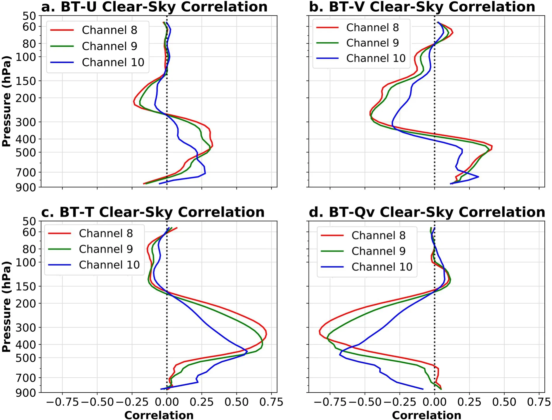
Fig.2.Time averages of the vertical correlations between the BTs and (a) U, (b) V, (c) T, and (d) Qv for clear-sky scenes.

Figure 5 shows the vertical correlations between the BTs and the atmospheric state variables for the high and low altitude cloud regions accompanied by the PDF of the CTPs for these two regions combined.A notable characteristic of Fig.5 is the different structures of correlations for the high altitude cloud region versus the low altitude cloud region across the three channels.In the high altitude cloud region, the correlations for different channels overlap with each other, unlike for the low altitude cloud region whose correlations are similar to those in the clear-sky region (Fig.2d),in the middle to upper troposphere.For the high altitude cloud region, BTs from all three channels are primarily determined by the cloud-top temperatures of these high clouds, leading to nearly identical BTs and correlations for the three of them.Cloud tops for columns in the low altitude cloud region are primarily at pressures greater than 700 hPa (Fig.5, black lines).These CTPs are much greater than the pressures at which the peaks of the weighting functions for the three channels occur.As a result, the low altitude clouds do not strongly impact the BTs of these three channels, with their BTs mostly a result of radiation originating from the troposphere above these low clouds.As a result, the structures and magnitudes of the correlations between the BTs and T and Qvin the low altitude cloud region (Figs.5c, d) are similar to those for the clear-sky scene (Figs.2c, d).The positive correlations in the lower troposphere between the BTs and Qv(Fig.5d, dashed lines),occurring at altitudes below those to which channels 8 and 9 are sensitive (Fig.3a), may be a result of the limited sample size for the low altitude cloud regions.

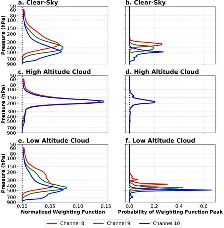
Fig.3.(a), (c), (e) Normalized averaged weighting functions and (b), (d), (f) PDFs of the peaks of the weighting functions of all the ensemble members for the three water vapor channels of ABI in (a), (b) clear-sky scenes, (c), (d) high altitude cloud regions, and (e), (f) low altitude cloud regions.

In both the high and low altitude cloud regions, correlations between the BTs and dynamic fields are again relatively weak (Figs.5a, b).Kerr et al.(2015) hypothesized that the feedbacks between the model dynamics and the storm environment may have produced the nonzero correlations between cloud-top temperatures and horizontal winds in their idealized supercell experiments.Peaks in the correlations between the BTs and T and Qvin the high altitude cloud region are located around 200 hPa (Figs.5c, d), near the cloud tops, and higher than for the low altitude cloud region and the clear-sky scenes (Figs.2c, d).Vertical correlations of BT with Qv(Fig.5d) are noticeably broader than those with T (Fig.5c) in the high altitude cloud region, probably because the underlying dynamics of moist convection in severe thunderstorms facilitate relationships between Qvand the BTs across a deeper range of the troposphere.A noticeable feature of the correlations between BT and T in the high altitude cloud region is a large spike at pressures just less than 200 hPa (Fig.5c).This spike is related to those in the normalized averaged weighting functions(Fig.3c) and the PDFs of the weighting function peaks(Fig.3d) of the high altitude cloud region because the BTs in this region are strongly modulated by the properties at cloud top.Because the BTs for columns in the low altitude cloud region are mostly sensitive to the clear-sky troposphere above the low altitude clouds, the weighting functions (Fig.3e) and the PDFs of the weighting function peaks(Fig.3f) in the low altitude cloud region are similar to those in the clear-sky scene (Figs.3a, b), although the PDFs are much noisier due to a much smaller sample size for the low altitude cloud region.The small sample size of the low altitude cloud region may also contribute to the positive correlations between Qvin the mid-troposphere and BT, which itself is a byproduct of a negative correlation between Qvin the upper troposphere and Qvin the middle troposphere.We would not expect this positive correlation to remain if a larger sample size covering more scenarios is used in the analysis.

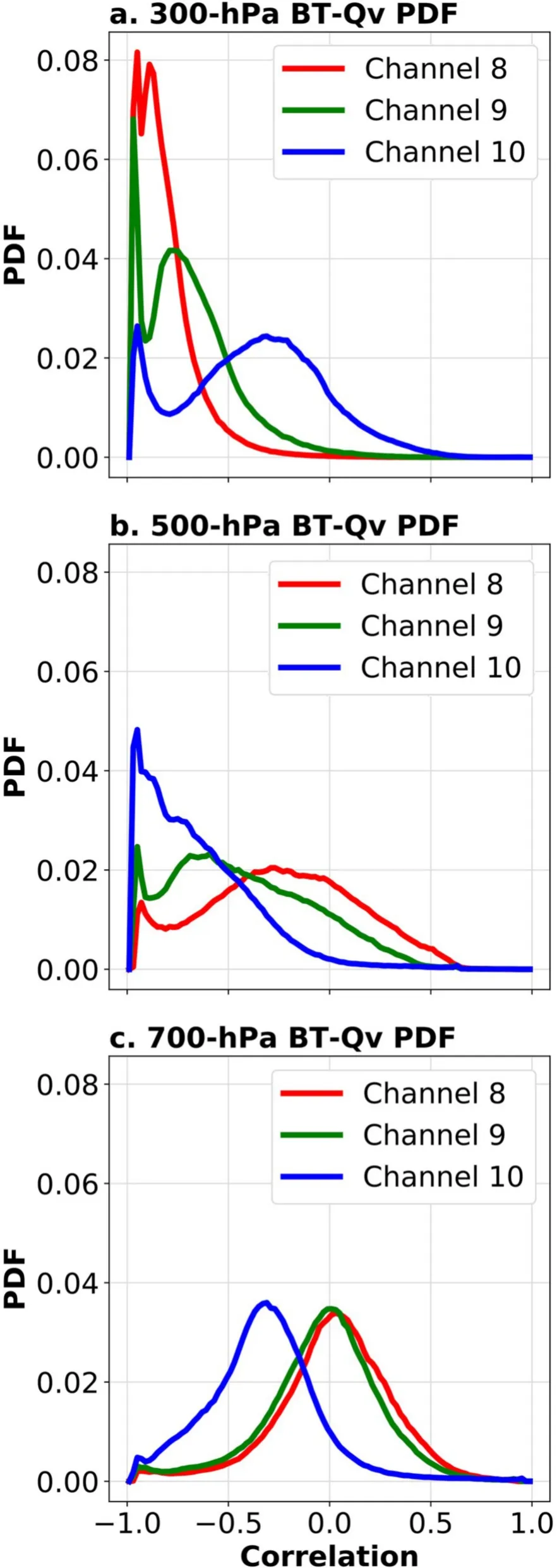
Fig.4.Time averages of the PDFs of the correlations between the BTs and the clear-sky scene BTs at vertical levels of (a) 300 hPa, (b) 500 hPa, and (c) 700 hPa.The narrow peaks in the PDF close to correlation values of −1,especially noticeable in (a) and (b), are the result of a deleterious impact of the boundary conditions along the southwestern corner of the model domain.

Hydrometeor mixing ratios exhibit negative correlations with BTs in the high altitude cloud region as more hydrometeors are often associated with higher (colder)cloud tops.Ice hydrometeors (cloud ice, snow, and graupel;Figs.5f, h, i) have stronger correlations than liquid hydrometeors (cloud liquid and rain; Figs.5e, g).Correlations with ice hydrometeors have peaks at 200 hPa (Figs.5f, h, i), consistent with the peak associated with Qvat cloud top (Fig.5d).The correlations with liquid hydrometeors peak around 300 hPa (Figs.5e, g).The stronger correlations with ice hydrometeors suggest potentially greater influences by them, as compared to the liquid hydrometeors, on the BTs.The correlations between the BTs and liquid hydrometeors at pressures greater than 300 hPa are not significantly weaker than those between the BTs and ice hydrometeors at these pressures.These results indicate that both the liquid and ice hydrometeors may have comparable contributions to the correlations at these lower altitudes, whereas the ice hydrometeors contribute greatest at the higher altitudes where liquid hydrometeor contents are low.The correlations between the BTs and all of the hydrometeors are weak and noisy in the low altitude cloud region (Figs.5e−i) because the BTs are most sensitive to the clear-sky layers above the low clouds.The definition of the low altitude cloud region ensures that the mixing ratios of all hydrometeors must be lower than 10−6kg kg−1at pressures less than 700 hPa.

Columns for the different cloud scenes and cloud structure regions discussed above are generally consistent within a scene or region type.Therefore, the structures in the correlations that result from them are generally well-defined and clearly associated with the underlying dynamic and thermodynamic processes.However, the structures in the correlations are more complex for partly cloudy scenes and mixed altitude cloud regions (Fig.6).PDFs of CTP for these scene and region types show that the mixed altitude cloud regions mostly contain hydrometeors with CTPs from about 150 hPa to 500 hPa (Fig.6, solid black lines).The partly cloudy scenes mostly contain clouds with CTPs at pressures greater than 600 hPa, together with some clouds with CTPs around 400 hPa (Fig.6, dashed black lines).During convection initiation, the timing of initiation and the development of clouds and precipitation vary considerably across ensemble members, leading to similar CTP PDFs like those in Fig.6.This time is also when the ensemble forecasts have some of their greatest uncertainties (e.g., Zhang et al., 2016b).Therefore,broad vertical correlations in the partly cloudy scenes and mixed altitude cloud regions come as no surprise.

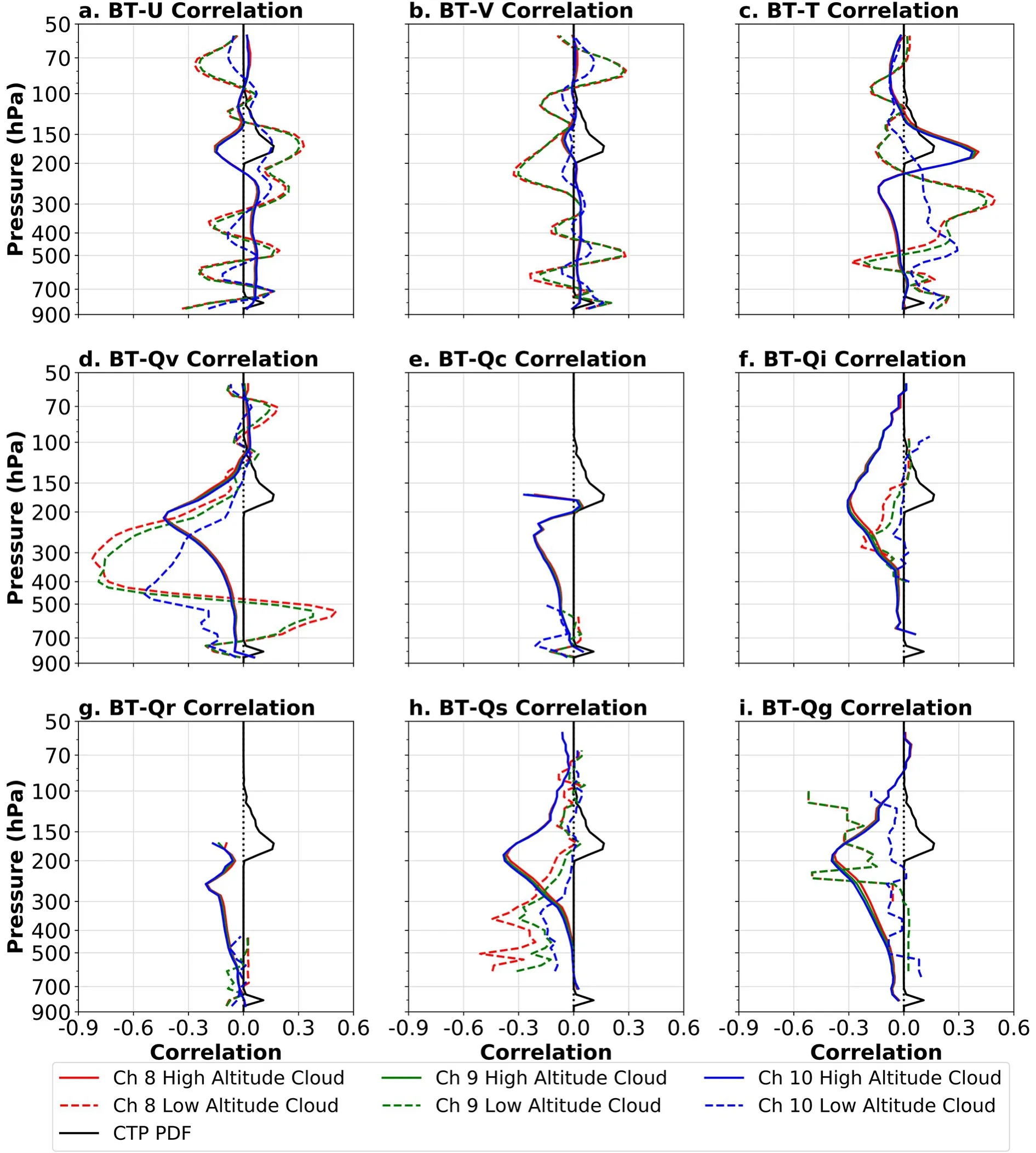
Fig.5.Time averages of the vertical correlations between the BTs and (a) U, (b) V, (c) T, (d) Qv, (e) Qc, (f) Qi, (g) Qr, (h) Qs,and (i) Qg for the high and low altitude cloud regions.The PDF of CTP for all member columns within either of the two cloud structure regions is illustrated by the same black line in all subpanels.

Compared with the correlations for the high altitude cloud regions, peaks in the correlations between the BTs and hydrometeor mixing ratios for the mixed altitude cloud regions move downward in altitude to around 300 hPa.This drop in altitude of the peak locations corresponds to the broader distribution of CTPs centered around 300 hPa for the mixed altitude cloud regions (Figs.6b−f).Peaks in the correlations of the BTs and Qvalso move downward.However,the altitudes of the peaks for the three channels are slightly different.Channel 8 has the highest altitude peak, and channel 10 has the lowest altitude peak (Fig.6a), although not as low as its peak for clear-sky scenes (Fig.2d).Considering that a notable number of the CTPs within the mixed altitude cloud regions are at pressures less than 500 hPa, the shifts of correlation peaks from channel 8 to channel 10(Fig.6a, solid-colored lines) suggest that the correlations in the mixed altitude cloud regions are averages of profiles that contain both high-altitude-cloud-like correlation profiles and low-altitude-cloud-like (and comparable to clearsky-like) correlation profiles.

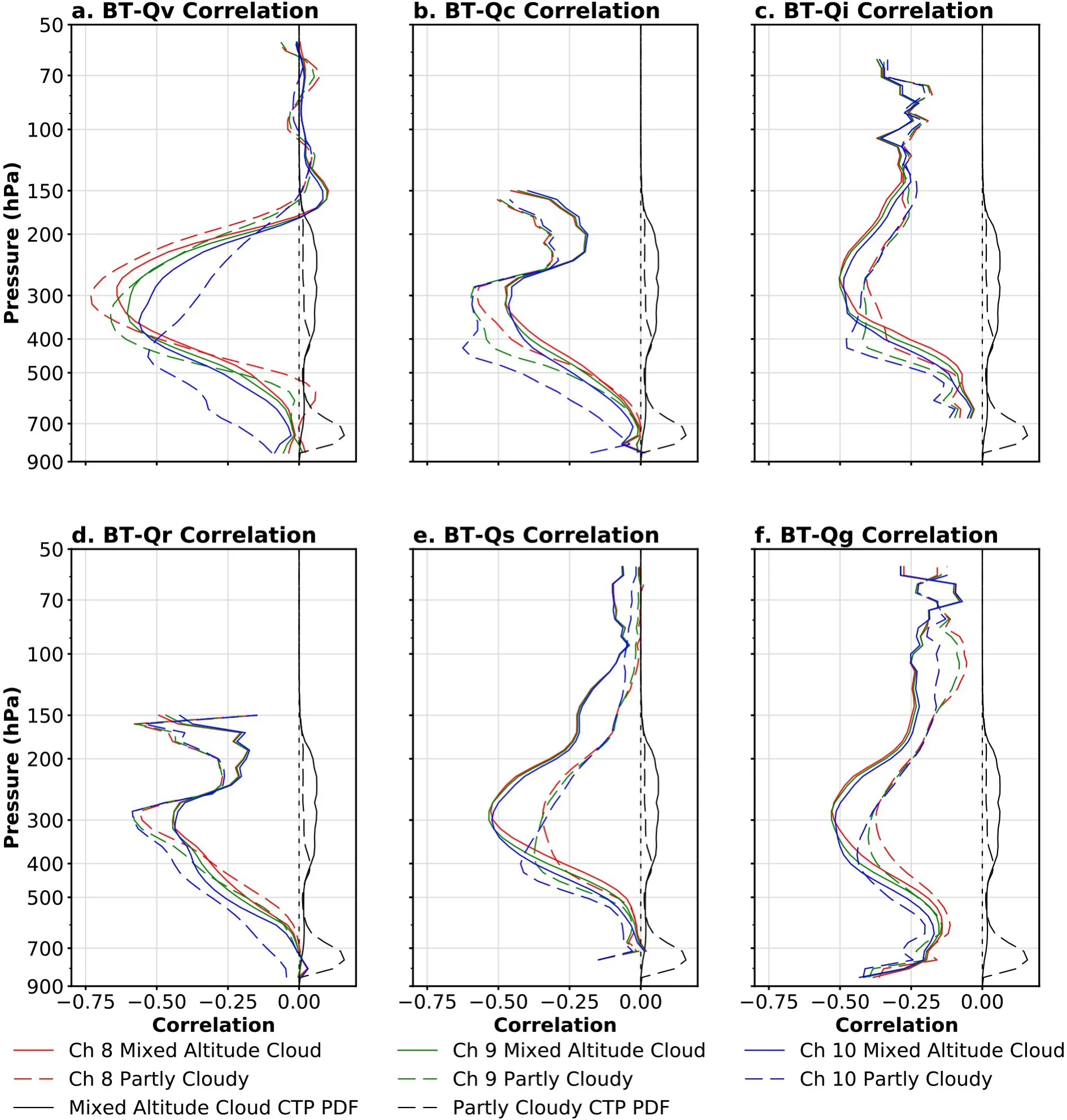
Fig.6.Time averages of the vertical correlations between the BTs and (a) Qv, (b) Qc, (c) Qi, (d) Qr, (e) Qs, and (f) Qg for partly cloudy scenes and mixed altitude cloud regions.The PDFs of CTP across all members are also illustrated for the partly cloudy scenes (dashed black lines) and the mixed altitude cloud regions (solid black lines).

The effect of this averaging is amplified for the partly cloudy scenes, where one correlation profile for a given column often contains contributions from ensemble members with and without clouds.With a considerable portion of CTPs at pressures greater than 600 hPa for the partly cloudy scenes, correlations with Qvare similar to those for the clear-sky scenes and the low altitude cloud regions.For the partly cloudy scenes, the correlations with the hydrometeors, except for Qr, show a similar shift in the vertical locations of their peaks.Moreover, the correlations with channel 10 BTs are stronger in magnitude in the lower troposphere compared with BTs from the other two channels.Unlike the low altitude cloud regions, the partly cloudy scenes contain a notable number of CTPs at pressures greater than 500 hPa, sufficient to produce reasonable correlations.

In short, we find that the vertical structures of correlations between the IR BTs and the atmospheric state variables depend on both the cloud scenes and the cloud structure regions, as well as consistency, or a lack thereof, across ensemble members of each type.We now examine how the correlations change with horizontal distance for different vertical levels in the atmosphere.

4.Horizontal structures in the correlations

We now focus on the change in the correlations between the BTs and the atmospheric state variables with respect to horizontal distance.Figure 7 shows time averages of the layer mean of the correlations between the BTs and Qvwith respect to horizontal distance at different vertical levels from 800 hPa to 100 hPa in 50 hPa steps for the clear-sky and fully cloudy scenes.We only show distances from 0 km to 150 km in the figure in order to better reveal details within 50 km.The leftmost column within each of the six panels in Fig.7, i.e., the averages of the absolute values of the correlations between the BTs and Qvvalues within 5 km horizontally of them, shows characteristics that are consistent with our analysis on the vertical structures in the correlations in the previous section.For example, for the clear-sky scenes, the strongest correlations for channels 8,9, and 10 appear at about 300 hPa, 350 hPa, and 450 hPa,respectively, and the strongest correlations in the fully cloudy scenes occur around 250 hPa for all three channels.As Fig.7 illustrates, the horizontal scales of the correlations for the clear-sky scenes are much longer than those for the fully cloudy scenes.The longest horizontal scales in the correlations appear in the upper troposphere.

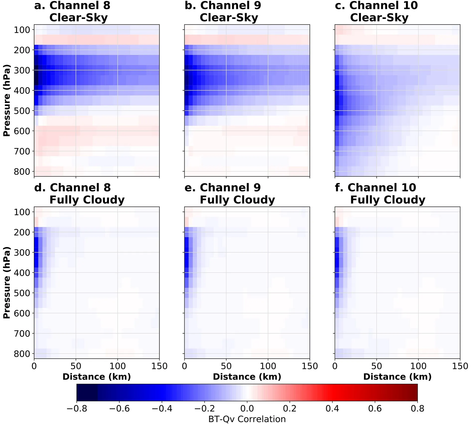
Fig.7.Time averages of the layer-mean correlations between the BTs and Qv with respect to horizontal distance for vertical levels from 100 hPa to 800 hPa in 50 hPa steps.The time averages are over all 21 EnKF data assimilation cycles for (a), (d)channel 8, (b), (e) channel 9, and (c), (f) channel 10 for (a), (b), (c) the clear-sky scenes, and (d), (e), (f) the fully cloudy scenes.

Correlations at 200 hPa, 300 hPa, and 450 hPa are shown in Fig.8 to facilitate further comparisons; the x-axis of Fig.8 has an upper limit of 300 km because the sample sizes with distances exceeding 300 km are very small.The 200-hPa pressure level is above all cloud tops, and channels 8 and 10 have maxima in their weighting functions near 300 hPa and 450 hPa, respectively.Consistent with our previous analysis on the vertical structures in the correlations (Fig.2d), for the clear-sky scenes, channels 8 and 9 have their strongest correlations at 300 hPa (Figs.8a, b),whereas channel 10 has its strongest correlations at 450 hPa for horizontal distances less than approximately 70 km(Fig.8c; where the yellow and pink lines intersect).The magnitudes of the correlations cease to decrease beyond approximately 100 km to 150 km, which is in agreement with the vertical mean absolute correlations (defined in section 2.3) for the clear-sky scenes (Fig.9a).The broad horizontal correlations between the BTs and Qvfor the clear-sky scenes result from the atmospheric state variables being more horizontally homogeneous in clear-sky scenes rather than in cloudy ones.This conclusion is also supported by Z21 who show that assimilating coarser spatial resolution BTs with broader localizations does not degrade the accuracy of the EnKF analysis for the clear-sky scenes.

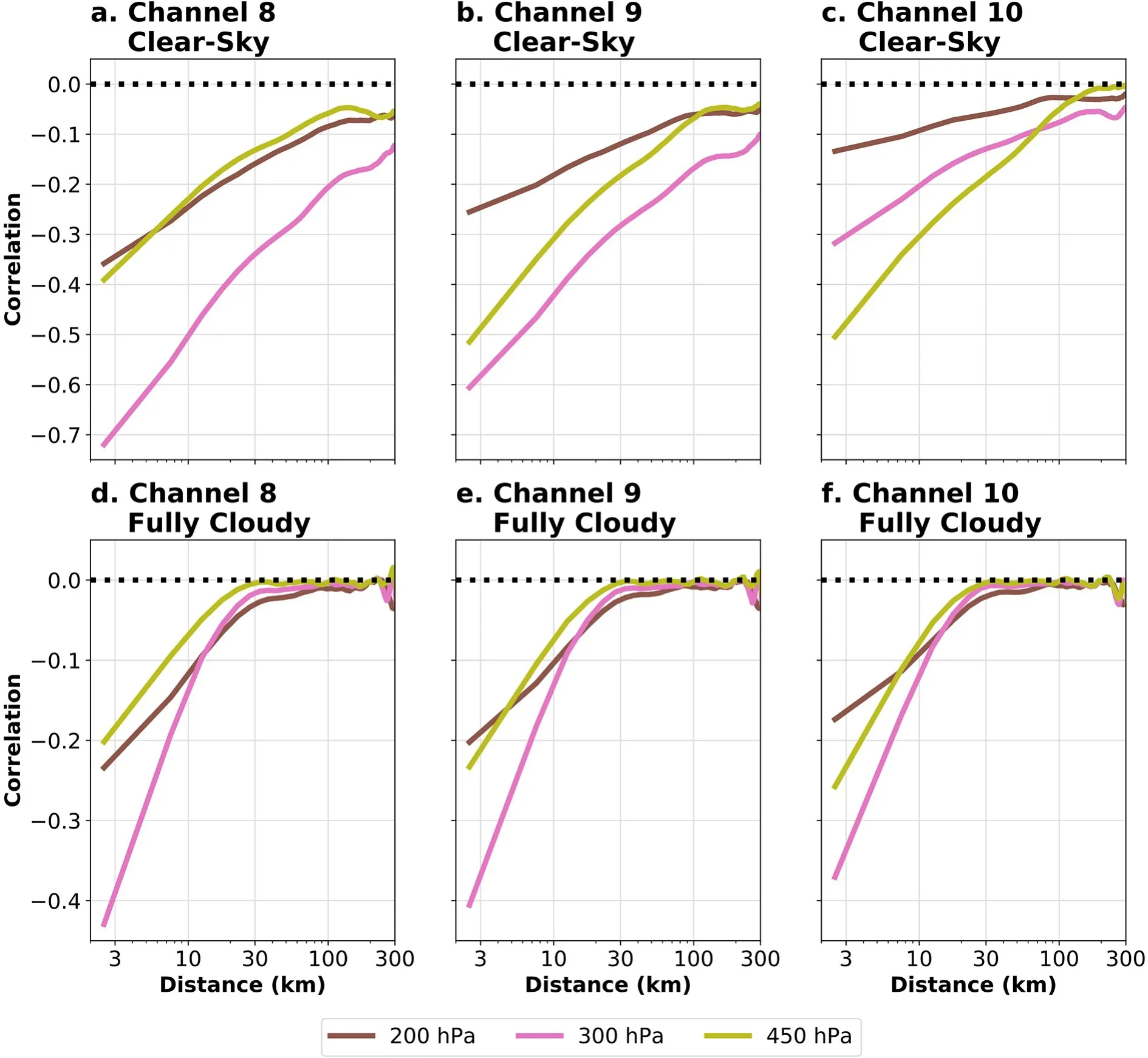
Fig.8.Time averages of the layer-mean correlations between the BTs and Qv with respect to horizontal distance.The time averages are over all 21 EnKF data assimilation cycles at 200 hPa, 300 hPa, and 450 hPa for (a), (d) channel 8, (b), (e)channel 9, and (c), (f) channel 10 for (a), (b), (c) the clear-sky scenes, and (d), (e), (f) the fully cloudy scenes.Correlations for horizontal distances longer than 300 km are omitted due to very small sample sizes of model grids at these distances.

For fully cloudy scenes, all three channels at the two vertical levels below cloud top show similar characteristics.The magnitudes of the correlations decrease rapidly with increasing distance and remain close to 0 when the distance exceeds about 30 km (Figs.8d, e, f and Fig.9c).The much shorter correlation length scale for the fully cloudy scenes is not surprising given that most dynamics within severe thunderstorms occur at similar or smaller scales.Because the correlations at 200 hPa for the fully cloudy scenes are for a vertical level above the cloud tops, slightly stronger correlations exist beyond 30 km (Figs.7d, e, f and Figs.8d, e, f).

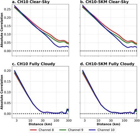
Fig.9.Averages over all 21 EnKF data assimilation cycles and all vertical levels of the absolute values of the layer-mean correlations between the BTs and Qv with respect to horizontal distance for (a), (b) the clear-sky scenes, and (c), (d) the fully cloudy scenes for the (a), (c) CH10 and (b), (d) CH10-5KM EnKF experiments.Correlations for horizontal distances longer than 300 km are omitted due to very small sample sizes of model grids at these distances.

Given that the horizontal ROI for the BTs in the EnKF data assimilation cycling of experiment CH10 is 30 km, we applied the same analysis on the results of another experiment from Z21, called the CH10-5KM experiment, that both the horizontal spacings and the ROI of the assimilated BTs are doubled compared with the CH10 experiment.The results obtained using the CH10-5KM experiment with a 60-km horizontal ROI (Figs.9b, d) are almost identical to those obtained using the 30-km ROI in the CH10 experiment (Figs.9a, c).These results suggest that the cut-off distance of 30 km is, at least for this event, inherent to the nature of the thunderstorms rather than modulated by the ROI applied during the EnKF data assimilation cycling.

The vertical mean absolute correlations between the BTs and hydrometeors for the fully cloudy scenes (Fig.10)are consistent with their vertical correlations (Fig.5).The correlations for the ice particles (i.e., cloud ice, snow, and graupel) are stronger than those for the liquid particles (i.e.,cloud liquid and rain).For all five hydrometeor species, the correlations drop to 0 at around 30 km (Fig.10), consistent with the correlations between the BTs and Qvfor the fully cloudy scene (Fig.9c).The consistency of the correlation cut-off distances between the BTs and the different atmospheric state variables for the fully cloudy scenes again reflect the scales of the underlying dynamical processes within this severe thunderstorm.

The correlations between the BTs and T for the clearsky scenes (Figs.11a, b, c) have similar structures with the correlations between the BTs and Qv(Figs.7a, b, c), except for being mostly positive and weaker in magnitude.These results, too, are consistent with the structures in the vertical correlations (Figs.2c, d).However, for the fully cloudy scenes,the magnitudes of the correlations between the BTs and T drop rapidly with distance for all vertical levels (Figs.11d,e, f).The vertical absolute mean correlations remain almost unchanged beyond 10 km (Figs.12d, e, f), noticeably shorter than the 30-km length scale of the correlations between the BTs and Qv.The correlations between the BTs and dynamical fields for the fully cloudy scenes remain unchanged beyond 30 km (Figs.12d, e, f), suggesting that this scale is once again associated with the storm dynamics.

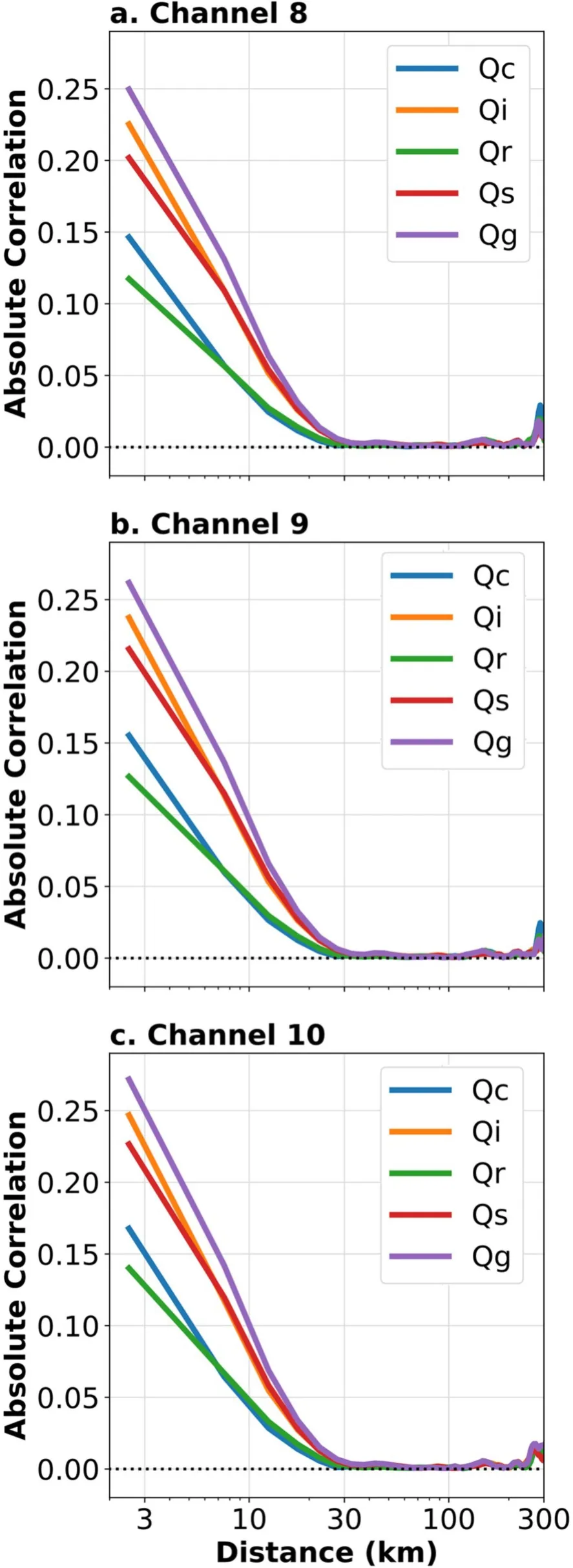
Fig.10.Averages over all 21 EnKF data assimilation cycles and all vertical levels of the absolute values of the layer-mean correlations between the BTs and hydrometeors with respect to horizontal distance for (a)channel 8, (b) channel 9, and (c) channel 10 for the fully cloudy scenes.Correlations for horizontal distances longer than 300 km are omitted due to very small sample sizes of model grids at these distances.

5.Summary

To address the problem of vertical localization of satellite radiance observations in an EnKF data assimilation system that has sampling errors resulting from limited ensemble size, we analyze EnKF experiments that assimilate conventional and satellite observations for the analysis and prediction of the tornadic supercell thunderstorm event on 12 June 2017 in the central United States.The horizontal and vertical structures in the correlations between infrared (IR) BTs observed by the three water vapor channels of the Advanced Baseline Imager (ABI) onboard the GOES-16 satellite and the atmospheric state variables are investigated in detail.The three ABI water vapor channels—channel 8 (6.2-μm wavelength), channel 9 (6.9-μm wavelength), and channel 10 (7.3-μm wavelength)—are sensitive to moisture within different layers of the troposphere,hence motivating our study of them.

Three cloud scenes—clear-sky, partly cloudy, and fully cloudy—are defined based on the probability of clouds.The fully cloudy scenes are further divided into three cloud structure regions—high altitude cloud, low altitude cloud, and mixed altitude cloud—based on the vertical distribution of cloud top pressure (CTP).Not surprisingly, the vertical structures in the correlations depend on the cloud scenes and the cloud structure regions.Under clear-sky conditions, vertical correlations between the infrared (IR) BTs and temperature (T), or moisture (Qv), resemble the structure of the BT weighting functions.Vertical correlations and the weighting functions of channel 8, channel 9, and channel 10 peak at approximately 320 hPa, 400 hPa, and 500 hPa, respectively.When moving away vertically from the level of the peak correlation for a channel, correlations generally become smaller in magnitude.Further examination of probability density functions (PDFs) of the vertical correlations between BT and water vapor mixing ratio (Qv) at three different vertical levels for each channel indicate a shift of the PDF peaks from negative values to approximately 0 with increasing vertical separation from the layers with the largest magnitudes, suggesting the existence of potentially spurious correlations.For example, PDFs of the correlations between ABI channel 8/9 and Qvat 700 hPa resemble a Gaussian distribution with a mean value of 0, implying that these PDFs of correlations are indistinguishable from random Gaussian noise.

In cloudy regions, the vertical correlations between BTs and atmospheric state variables are determined by both the structures of the clouds and their coherence across the ensemble members.When all ensemble members contain high clouds (i.e., high altitude cloud regions within fully cloudy scenes), the BTs are mostly sensitive to the atmospheric state at cloud top and more sensitive to ice hydrometeors (i.e., cloud ice, snow, and graupel) than liquid hydrometeors (i.e., cloud liquid and rain).For these high altitude cloud regions, little difference exists across the three ABI water vapor channels.When all ensemble members contain low clouds (i.e., low altitude cloud regions within fully cloudy scenes), all of which are well below the altitudes at which the weighting functions of the ABI water vapor channels peak, the BTs are mostly sensitive to the troposphere above these clouds.For these low clouds, the vertical structures in the correlations resemble those under clear-sky conditions.However, a more common situation in an EnKF approach to severe storm forecasting, especially during convection initiation, is a combination of clouds at different heights (i.e., mixed altitude cloud regions within fully cloudy scenes) or a combination of cloudy and clear-sky conditions across the members (i.e., partly cloudy scenes).For these cases, the vertical structures in the correlations become combinations of high altitude cloud correlation profiles and clear-sky correlation profiles, depending on the specific combination of cloud scenes and/or cloud structure regions.This makes correlation localization in the vertical direction more ambiguous in these regions.

The horizontal structures in the correlations contain some of the characteristics of the vertical structures in the correlations.For example, the largest magnitude correlations generally occur either at the heights of the weighting function peaks in clear-sky or low altitude cloud columns or at cloud top in high altitude cloud columns.The magnitudes of the correlations decrease with increasing horizontal separation between the BT column and the column of the atmospheric state variables.The reductions in the magnitudes of the correlations with distance are slower for clear-sky scenes compared with fully cloudy scenes.The horizontal cut-off distance (a.k.a., radius of influence) of the correlations, or the distance beyond which the magnitudes of the correlations cease to decrease, is much broader for the clear-sky scenes(~100 km) than the high and mixed altitude cloud regions of the fully cloudy scenes (~30 km).This difference between the cut-off distances of the correlations in clear-sky scenes versus fully cloudy scenes is not surprising, given that the atmospheric state variables for the clear-sky scenes are usually more homogeneous than for fully cloudy regions,where large spatial variabilities in the atmospheric state variables exist.The horizontal correlations between the BTs and the hydrometeors, as well as the dynamical fields, also consistently exhibit this 30-km cut-off distance in fully cloudy scenes, implying that this length scale may be inherently determined by the scale of the underlying dynamic and thermodynamic processes of the severe thunderstorms examined in this study.

The results of this study provide information on the localization of all-sky IR BTs in both horizontal and vertical directions for convection-allowing regional EnKF applications,although we must be cautious in generalizing results from the single case period in this study.For horizontal localization, a much broader ROI, together with less dense BTs is appropriate for clear-sky scenes as compared to cloudy ones.This result is also supported by Z21 who found that using thinned BTs with enlarged ROIs does not degrade the accuracy of the analysis in clear-sky scenes.For vertical localization, schemes based on the vertical structures in the correlations and/or weighting functions of each channel appear to be appropriate, in which the weighting functions facilitate adaptively assigning pseudo heights to each of the BTs.In fact, the global group filter (GGF) that is used to generate vertical localization functions in Lei et al.(2020) has shapes similar to the absolute values of the vertical correlations.Their fitted Gaspari−Cohn localization function shares the same vertical peak location with that of the vertical correlations.Other techniques, such as sampling error correction (SEC;Anderson, 2012) is also applicable in tandem with vertical localization as it loosens accuracy requirements in the estimation of the vertical ROI.The vertical structures in the correlations also suggest the potential of assimilating multiple IR channels over clear-sky scenes when proper vertical localization is applied, in which case each channel will impact a different layer of the troposphere to which it is most sensitive.Assessing the value of ABI channel 9, whose weighting functions have significant overlap with those of ABI channels 8 and 10, is a natural next step.With appropriate vertical localizations for each channel, a more accurate analysis throughout the entire troposphere should be attainable in comparison to when only one channel is assimilated.

Our analysis also reveals that constraining boundary layer clouds using any of the water vapor channels examined in this study may be problematic because the weighting functions for all three channels peak at altitudes much higher than these clouds.Boundary layer clouds are sometimes associated with structures such as gust fronts that are precursors of subsequent convection initiation, so information about these low clouds is of value in data assimilation.Whereas the ABI IR water vapor channels may not provide useful information on boundary layer clouds, ABI’s IR window channels or visible channels may.For assimilation of the IR window channels, large errors in the model surface emissivity and/or model surface temperature will deleteriously impact the modeled radiative transfer calculations,potentially limiting the value of direct assimilation of observations from these channels.To circumvent these problems,new methods need to be advanced, such as the channel synthesizing technique proposed by Lu and Zhang (2018).To advance assimilation of visible channel radiances, Scheck et al.(2020) and Schröttle et al.(2020) have incorporated features into the forward radiative transfer operator that facilitates the assimilation of visible reflectances, during the daytime, into a NWP model.How to best constrain cloud fields,especially for boundary layer clouds, using a combination of different channels deserves further investigation.

Acknowledgements.This article is dedicated to Dr.Fuqing ZHANG, who was a talented mentor, a wonderful colleague, and a very good friend.The authors would like to thank Dr.Yinghui LU of Nanjing University for his help on the CRTM model, and a reviewer who helped us to improve the clarity of this paper.This work is supported by the NASA under awards NNX15AQ51G and 80NSSC19K0728, the ONR under award N000141812517, and the NOAA Office of Weather and Air Quality under award NA18OAR4590369.The numerical experiments were performed on the Stampede 2 supercomputer of the Texas Advanced Computing Center (TACC) through the Extreme Science and Engineering Discovery Environment (XSEDE) program of the National Science Foundation (NSF).

Open AccessThis article is licensed under a Creative Commons Attribution 4.0 International License, which permits use, sharing, adaptation, distribution and reproduction in any medium or format, as long as you give appropriate credit to the original author(s) and the source, provide a link to the Creative Commons licence, and indicate if changes were made.The images or other third party material in this article are included in the article’s Creative Commons licence, unless indicated otherwise in a credit line to the material.If material is not included in the article’s Creative Commons licence and your intended use is not permitted by statutory regulation or exceeds the permitted use, you will need to obtain permission directly from the copyright holder.To view a copy of this licence, visit http://creativecommons.org/licenses/by/4.0/.