部分可观测耦合随机抛物方程组的参数估计

苗菲菲

(四川大学数学学院, 成都 610064)

1 Introduction

The general analytical theory of (linear and nonlinear) stochastic partial differential equations (SPDE) has made great progress and become a mature mathematical field in the past few decades. Stochastic partial differential equations (SPDEs) generalize deterministic partial differential equations (PDEs) by introducing driving noise processes into dynamics. Not only the theory of SPDEs, but also the statistics for SPDEs have recently seen a significant development, paving the way for a realistic modeling of complex phenomena.

The SPDE interested in this paper belongs to a general class of activator-inhibitor models, which can be described by two coupled stochastic reaction-diffusion equationsX=(A,I) of the following form:

whereX=(A,I), with space-time white noise processesξA,ξI, andσA,σIare the noise levels. In cell dynamics, we think ofAas a hypothetical signalling molecule in response to an external signal gradient becoming enriched on one side of the cell with diffusionDA, yielding polarity.Icounter-actsAso that removal of the signal results in loss of polarity with diffusionDI.fAandfIrepresent the interaction functions of activatorAand inhibitorI. More detailed information aboutfAandfIcan be found in Ref.[1]. Meinhardt[2]has been the first to apply such models to cell polarisation in the context of cell migration, where the ratio of activator-inhibitor diffusion can be tuned to either obtain a single stable cell front, or multiple independent fronts associated with non-directed random cell motility.

In the current paper we present a simple version of the modified Meinhardt two variable model. We setfA(X(t,x),x)=I(t,x),fI(X(t,x),x)=A(t,x),σA=σI=1,DI=1 and focus on the following specific coupled stochastic parabolic equations problem:

where Λ=(0,π), {W1(t)}t≥0and {W2(t)}t≥0are two cylindrical Brownian motions onL2(Λ), (dWi(t,x),i=1,2 is also referred to asspace-timewhite noise) on a complete filtered probability space=(Ω,F,{Ft}t≥0,) with the usual assumptions (completeness ofF0and right-continuity ofFt),T<∞ is fixed, moreover,θ∈(α,β),α>0 is the unknown parameter to be estimated based on finite dimensional approximations to solutions of such systems.

To the best of our knowledge, this problem has not been studied for the partially observable coupled stochastic parabolic equations, that is to say, we can only observe one process in the coupled equations. In this paper, we extend the estimation method introduced by Huebner and Khasminskii[3], where the parameter estimation in a single equation is discussed and first introduced by using the spectral method to study the consistency, asymptotic normality and asymptotic efficiency of maximum likelihood estimator of a parameter in the drift coefficient of an SPDE. Recently, Cialenco[4]showed some attractive methods to estimate parameters in stochastic partial differential equations. Most approaches focus on estimating coefficients for the linear part of the equation, either from discrete[5]or spectral observations[3, 6], but also the aspects of the driving noise[7, 8], have been analysed.

The paper is organized as follows. In Section 2 we set the stage: starting with notations, continuing with the solution of Eq.(1), ending with the description of the statistical experiment and presenting the main object of this study: the maximum likelihood estimator. Section 3 is dedicated to the main results. Numerical example which illustrate the efficiency of the proposed estimator are presented in Section 4.

2 Preliminaries

For a random variableξ,ξand Varξdenote the expectation and the variance, respectively.Rnis ann-dimensional Euclidean space,N(m,σ2) is a Gaussian random variable with meanmand varianceσ2.B*denote the transpose of matrixB. Notationan～bnfor two sequences, withan>0,bn>0, means thatFor example ,n2-2n～n2and

Let us look for the solution of Eq.(1) as a Fourier series.

Definition2.1A solution of Eq.(1) are two random element with values inL2((0,T)×Λ), such that, for every twice continuously differentiable on [0,π] functionφ(x) satisfyingφ(0)=φ(π)=0 and everyt∈[0,T], the following equality holds with probability 1:

Proposition2.2There exists a unique solution of Eq.(1).

where{Wi,k(t)}k≥1,i=1,2 are independent standard Brownian motions for differentk. We find thatuk(t)=(u,hk)L2(Λ)(t) andvk(t)=(v,hk)L2(Λ)(t) satisfy

(3)

Denote

and

We know the solution of thisYk(t) is

(4)

hereVkis a two-dimensional standard Brownian motion. Therefore,

(5)

where

and

By calculation, we have

(6)

and

(7)

Sincehk,k≥1 is an orthogonal basis inL2(Λ), we conclude thatu=∑k≥1ukhkandv=∑k≥1vkhkare solutions of Eq.(1). Uniqueness of solutions of Eq.(1) follows from the uniqueness of solution of Eq.(3) for everyk. Proposition 2.2 is proved.

(8)

MaximisingLN(θ) with respect toθ, leads to the following MLE :

(9)

3 The main results

(10)

Also it is a asymptotically normal estimator ofθ, that is,

(11)

Lemma3.2[10]Letξn,n≥1 be independent random variables such thatξn≥0, ∑k≥1ξk=+∞, and

Then

with probability one.

Lemma3.3[10]Letwk=wk(t),k=1,...,nbe independent standard Brownian motions and letfk=fk(t),k=1,...,nbe adapted, continuous, square-integrable processes such that

in probability. Then

ProofofTheorem3.1We borrow some ideas from Lototsky[10]. From Eq.(8), we can get

(12)

(13)

(14)

From now on, we divide the proof into two parts. At first, we prove that

(15)

in probability. Next, we prove

(16)

in probability.

(i) In order to estimate Eq.(14), we firstly do some computations. we have

(17)

(18)

and

(19)

(20)

Next by applying Lemma 3.2, the following equality

(21)

holds in probability. Further, combining Eq.(5)and Eq.(16), we have

(22)

Now we estimate

(23)

from Eq.(13) and obtain

(24)

The last equality can be derived from Eq.(6). On the other hand, the Cauchy-Schwarz inequality shows that

(25)

Eq.(23) and Eq.(24) lead to

(26)

Finally, it holds that

(27)

Combining Eq.(20), Eq.(21) and Eq.(26), Eq.(14) holds in probability.

(ii) According to Eq.(22)～Eq.(26), one can also get

(28)

From Eq.(16), we have

(29)

and

(30)

By applying Lemma 3.2, the following equality

(31)

holds in probability. Moreover, forv(t,x), we can take the same separation asu(t,x), then we have

(32)

As the same asuk(t), forvk(t), we have

and

(33)

Substituting these equalities and Eq.(14), Eq.(27), Eq.(30) into the inequality below, it is direct to obtain that

Then, by

together with Eq.(16), one has

in probability. Thus Eq.(15) holds. Substituting Eq.(14) and Eq.(15) into Eq.(11), we obtain

(34)

By direct calculating with Eq.(5), we obtain

Therefore，

Furthermore， one also has

Eq.(10) holds. The proof is end.

4 A numerical example

Tab.1 The ME and MSE of MLE

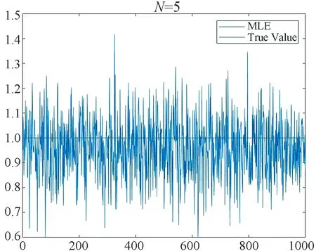
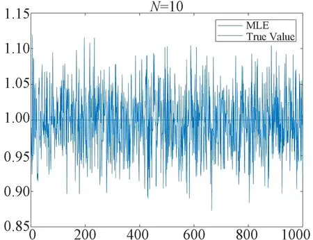
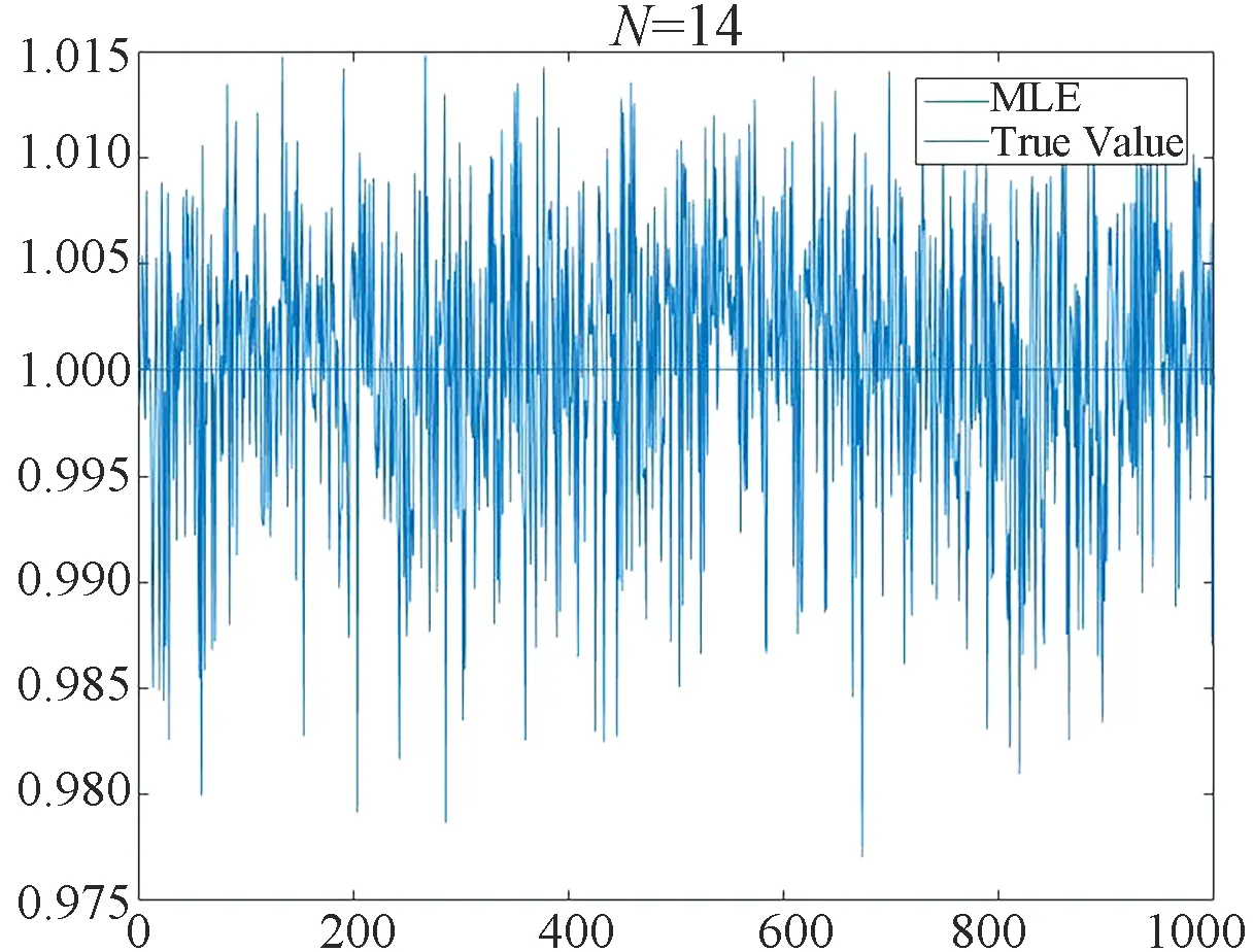
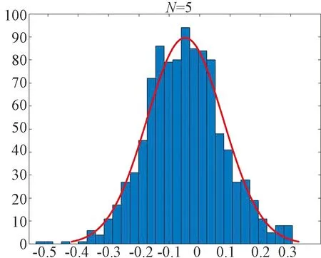
Fig.1～Fig.4 are plotted under the setting (ii). Fig.1 shows the MLEand the true value on one picture withN=5,N=10 andN=14. We find that asNincreases, MLEis closer to the true value. Fig.2 depicts the histogram of the statisticwithN=5,N=10 andN=14. The dashed curve is the normal density. Fig.3 depicts the histogram of the statisticwithN=14. Fig.4 we use the normplot function in matlab to compares the distribution of the data ofto the normal distribution withN=5,N=10 andN=14, we can find that the coincidence degree is very high.

(a)

(b)

(c)

(a)

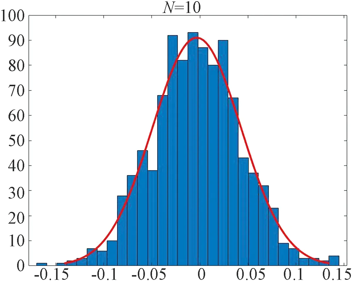
(b)

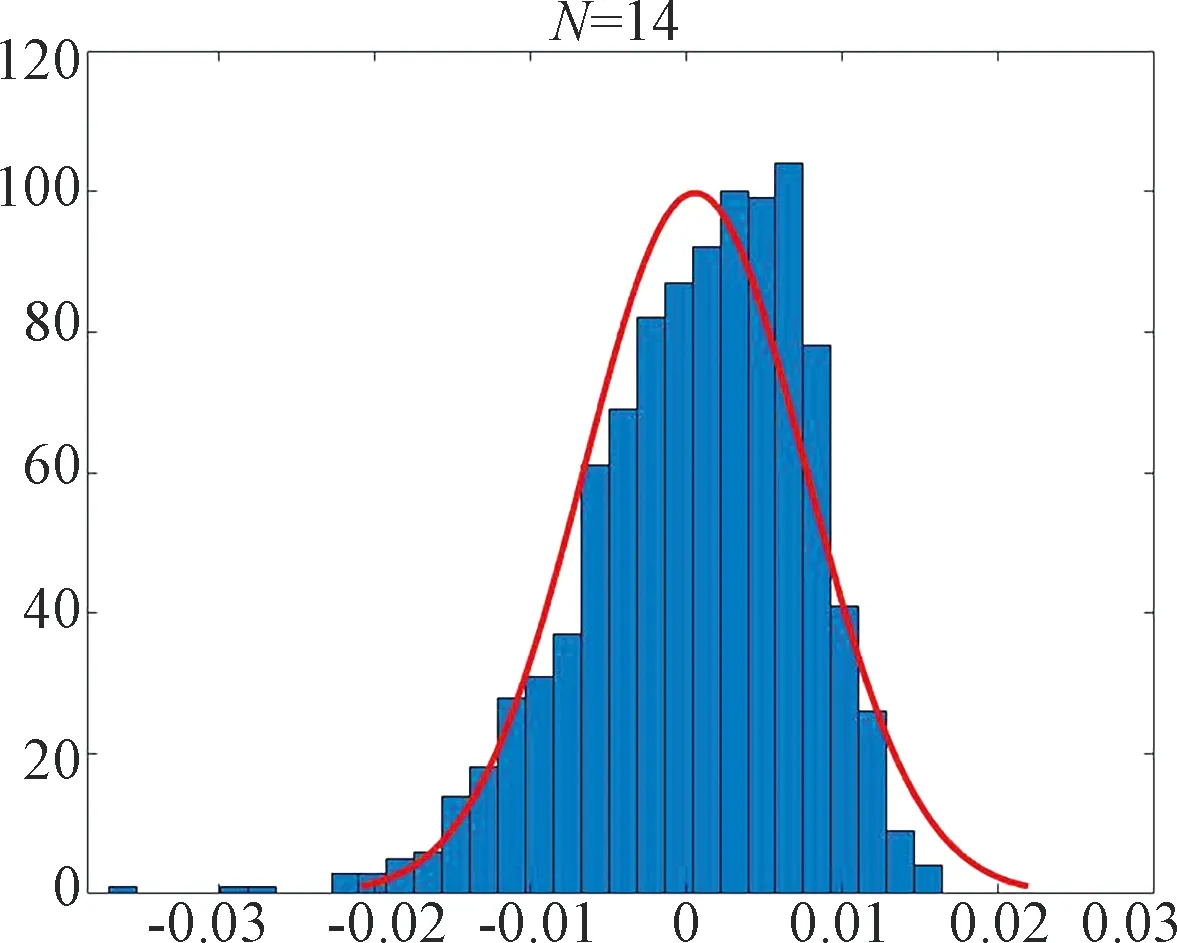
(c)

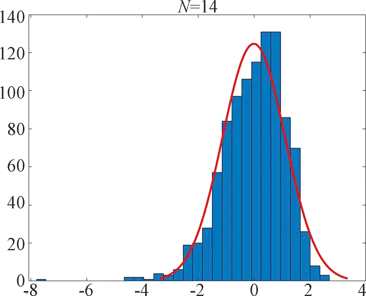
Fig.3 Histogram of with N=14. The curve is plot of the normal density: μ= -0.013 475 1 [-0.082 977 3, 0.056 027 2], σ= 1.120 02 [1.072 99, 1.171 39]

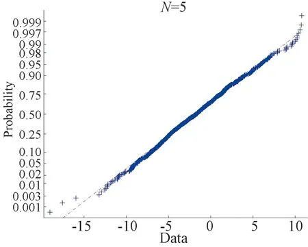
(a)

(b)

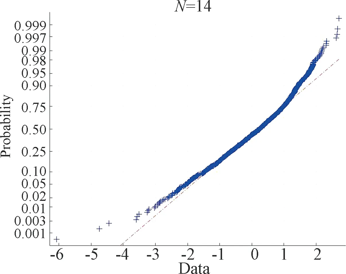
(c)