Data-Driven Discovery of Stochastic Differential Equations

Ysn Wng, Huzhn Fng, Junyng Jin, Guijun M, Xin H, Xing Di,,Zuogong Yu, Chng Chng, Hi-To Zhngb,, Donglin Pu, Dongrui Wu, Y Yun,,*,Jorg Gonçlvs,f,g, Jürgn Kurths, Hn Ding,

aSchoolofMechanicalScienceandEngineering,HuazhongUniversityofScienceandTechnology,Wuhan430074,China

bStateKeyLaboratoryofDigital ManufacturingEquipment andTechnology,HuazhongUniversityofScience andTechnology,Wuhan430074,China

c Department ofMechanicalEngineering,Universityof Kansas, Lawrence,KS66045,USA

d HUST-WuxiResearchInstitute,Wuxi 214174,China

eKeyLaboratory ofImageProcessingandIntelligentControl,SchoolofArtificialIntelligence andAutomation, HuazhongUniversityofScienceandTechnology, Wuhan 430074, China

fDepartmentofPlant Sciences, UniversityofCambridge, CambridgeCB23EA, UK

gLuxembourg CentreforSystemsBiomedicine, UniversityofLuxembourg,Belvaux4367, Luxembourg

h Department ofPhysics,HumboldtUniversityof Berlin, Berlin12489,Germany

i DepartmentofComplexityScience,PotsdamInstitutefor ClimateImpactResearch,Potsdam14473,Germany

Keywords:Data-driven method System identification Sparse Bayesian learning Stochastic differential equations Random phenomena

A B S T R A C T Stochastic differential equations (SDEs) are mathematical models that are widely used to describe complex processes or phenomena perturbed by random noise from different sources. The identification of SDEs governing a system is often a challenge because of the inherent strong stochasticity of data and the complexity of the system’s dynamics.The practical utility of existing parametric approaches for identifying SDEs is usually limited by insufficient data resources. This study presents a novel framework for identifying SDEs by leveraging the sparse Bayesian learning(SBL)technique to search for a parsimonious,yet physically necessary representation from the space of candidate basis functions. More importantly,we use the analytical tractability of SBL to develop an efficient way to formulate the linear regression problem for the discovery of SDEs that requires considerably less time-series data. The effectiveness of the proposed framework is demonstrated using real data on stock and oil prices, bearing variation, and wind speed, as well as simulated data on well-known stochastic dynamical systems, including the generalized Wiener process and Langevin equation. This framework aims to assist specialists in extracting stochastic mathematical models from random phenomena in the natural sciences, economics, and engineering fields for analysis, prediction, and decision making.

1. Introduction

Nature,industry,and human society are teeming with phenomena,processes,and systems that evolve with the effects of random noise. Examples of such systems include the motion of Brownian particles in a fluid [1], evolution of tumors driven by tumorimmune interactions [2], price of stocks, and movement of winds.Stochastic differential equations (SDEs) are a powerful mathematical approach for modeling and analyzing systems affected by random noise. The study of SDEs originates in one of Einstein’s annus mirabilis papers [1], which theorizes the fluctuation of Brownian particles in a thermal bath.Since then,the application of SDEs has spread across numerous scientific and engineering fields [3–7]. Traditionally, SDEs have been employed to model random phenomena based on the statistical properties of data or the experience of specialists. However, in many cases,the statistical properties of data may not resemble those of wellunderstood SDEs, and are thus less helpful for the discovery of underlying SDEs.Additionally,the governing SDEs of random phenomena are typically unknown or elusive.Therefore,it is crucial to develop a data-driven method for identifying the underlying SDEs of random phenomena.However,the complex behavior and strong stochasticity often present in SDE-governed systems makes the accurate identification of SDEs particularly challenging.

The key to determining an SDE is the identification of its drift and diffusion terms. The growing body of work on this subject can be roughly divided into two categories. The first lies in nonparametric identification, which seeks to build a model-free input–output mapping for drift and diffusion terms from timeseries data. The Kramers–Moyal average introduces histogrambased regression (HBR) to formulate a suitable mapping for the drift and diffusion terms[8].However,this method requires a large amount of data even for one-dimensional SDEs, and the required amount of data increases exponentially with the SDE’s dimensionality.Realistically,this data requirement aggravates the burdens of sensor cost,data storage,and computational resources,which may be difficult to meet in some cases. To improve identification accuracy with a limited amount of data, kernel-based regression(KBR)[9] and polynomial-based method [10] have been proposed as more efficient mapping methods for one-dimensional SDEs. In addition, non-parametric Bayesian estimation provides another mapping approach to mitigate the high demand for time-series data [11–14]. Markov chain Monte Carlo (MCMC) methods[11,12] and Gaussian process regression (GPR) [13] have recently been proposed for the identification of SDEs. Furthermore, sparse GPRs have been developed to learn SDEs with high computational efficiency [13,14]. While the aforementioned methods can predict drift and diffusion terms adequately,they cannot model stochastic dynamical systems because they only provide black-box representations.

In contrast, parametric approaches focus on identifying the model structures of the drift and diffusion terms of an SDE, and are more advantageous in revealing the underlying physical laws of stochastic dynamical systems. For scalar homogeneous SDEs with known model structures,the KBR and least-squares methods are combined to estimate parameters[15].For non-linear dynamical systems,a framework called sparse identification of non-linear dynamics (SINDy) has been applied to determine governing equations under the assumption that the model structure is sparse in the space of possible basis functions[16].Based on HBR and SINDy,sparse learning approaches have been proposed to identify drift and diffusion terms [17,18]. However, these approaches exhibit the same drawbacks as HBR because they initially rely on HBR to estimate the drift and diffusion terms.

An emerging technique for identifying model structures in the fields of system identification and signal processing is sparse Bayesian learning (SBL) [19–25], which aims to find a parsimonious representation from basis functions based on input–output data by striking a balance between model complexity and accuracy. The present study leverages this technique to discover the underlying SDEs of stochastic dynamical systems using relatively limited time-series data. The implementation of the proposed algorithm can be summarized in terms of the following two stages. First, theoretical expressions for the drift and diffusion terms are derived by discretizing SDEs with the Euler–Maruyama method. Then, the discovery problem of SDEs is cast into an input–output regression problem for the drift and diffusion terms based on the central limit theorem. Although the binning operation can be used to estimate the values of the drift and diffusion terms at the selected point to formulate the input–output regression problem, this operation is data-hungry and suffers from the curse of dimensionality. Owing to the analytical tractability of SBL, a more efficient method that can be implemented using relatively limited quantities of time-series data in practice is proposed herein. The enhanced capabilities and robustness of the proposed algorithm, named Bayesian identification of SDEs(BISDEs), were demonstrated on well-known SDEs against those of the state-of-the-art method. Additionally, the proposed BISDE algorithm was validated over a wide range of simulated and real-world systems.

2. Methods

2.1. Mathematical expressions for the drift and diffusion terms

In this study, we consider the n-dimensional SDEs in a general form as follows:

where x(t )∊Rnis the state vector at time t,f (x(t ))∊Rnis the statedependent drift vector, G(x(t ))∊Rn×nis the positive-definite diffusion matrix,and W t( )is an n-dimensional standard Brownian motion or Wiener process.It is assumed that each entry for f (x(t ))and G (x(t ))is a continuous function. However, the exact model structures for f (x(t ))and G(x(t ))are unknown.The objective of this study is to identify them from the relatively limited time-series data of x(t ).

Because analytical solutions for SDEs are generally unavailable,we resort to the Euler–Maruyama discretization. To ensure the existence and uniqueness of the solution of the SDE in Eq. (1)and the feasibility of the Euler–Maruyama method,we assume that the drift and diffusion terms satisfy the local Lipschitz and Khasminskii-type conditions (Section S1 in Appendix A). Furthermore, under these conditions, the numerical solution based on the Euler–Maruyama method converges to the exact solution in probability [26,27].

Applying the Euler–Maruyama method to the SDE in Eq.(1),we have

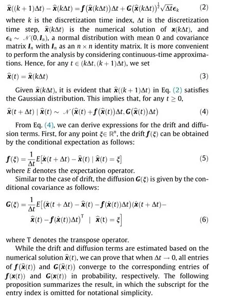
Proposition 1.Suppose that the SDE in Eq.(1)satisfies the local Lipschitz and Khasminskii-type conditions, and each entry of the drift and diffusion terms is a continuous function. Then, for any τ>0,

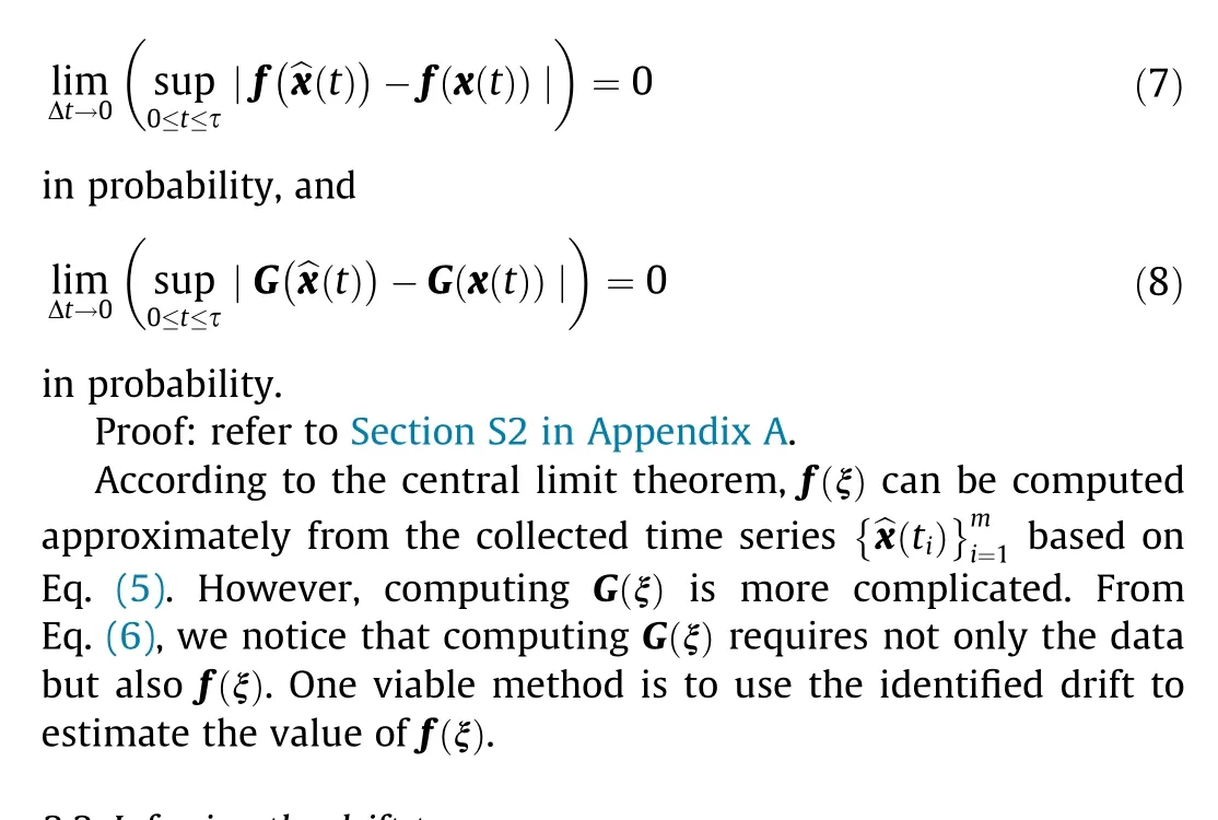
2.2. Inferring the drift term

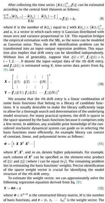
Proof: refer to Section S2 in Appendix A.

2.3. Inferring the diffusion term

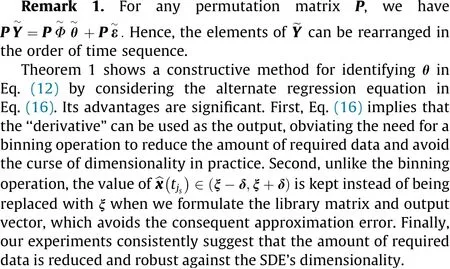
Once the drift is successfully identified, a regression equation can be formulated to identify the diffusion term. Based on Eq. (6)for diffusion, we consider

where ε2is a matrix with each entry being Gaussian distributed with mean zero and variance proportional to 1/K. The identified drift was used to estimate the corresponding exact drift value. Following similar lines as in the identification of the drift, we can formulate a regression equation to identify the diffusion term and leverage the SBL approach to solve it. Note that the selection of basis functions here can be different from those used for drift identification.

2.4. Model validation

Next, we evaluated the proposed BISDE algorithm through simulations and experiments. For simulations, because the exact model structures are known, we can compare the mean squared error (MSE) between the data generated by the true drift (diffusion)and the fitted drift(diffusion)at the measurements to assess the identified models’ performance. For real experimental data,owing to the absence of ground truth, we designed three criteria to assess the identified models’ performance.

Criterion 1: If a widely accepted model exists, we can leverage it to assess the identified model. If a good consistency is found between them, the effectiveness of such a model is cross verified.Otherwise, obvious inconsistency may imply the potential to determine a more efficient model whose performance can be assessed by Criteria 2 or 3.

Criterion 2: If the real dynamic process is approximately stationary, we can compare the analytic probability density function(PDF) of the identified model derived by solving the stationary Fokker–Planck equation with the empirical PDF of the timeseries. A good match between them suggests the soundness of identification. Non-stationary processes can be transformed into stationary processes by constructing algebraic or logarithmic increments, or by other methods [28].

Criterion 3: When the PDF cannot be solved analytically or estimated numerically for stationary processes, we can run the identified model with initial conditions identical to those of real data, and then assess the identified model’s performance by comparing the empirical PDF of the simulated data to that of the real data.

3. Results

3.1. Discovering the Langevin equation using simulated data

We first applied the proposed BISDE algorithm to the Langevin equation (Section S3.1 in Appendix A), which plays an important role in physics[29,30],as shown in Fig.1.Despite its simple mathematical form,it took physicists nearly a hundred years to discover this equation. Specifically, the Langevin equation describes the dynamics of Brownian particles over all time scales, which overcomes the shortcomings of Einstein’s theory in Ref. [1]. Consider a Brownian particle immersed in a fluid (Fig. 1(a)). Its random movements are driven by collision with liquid molecules from all directions due to thermal motion, and its velocity follows the Langevin equation.

The data were obtained by uniformly discretizing the time interval [0, 1000] with a time step Δt =0∙04. The basis functions consist of the constant term, polynomials in x up to the order of 15,and exponential functions with exponents from x to 10x.In this example, the same basis functions were employed for both drift and diffusion identification. If prior information relating to drift or diffusion, such as symmetry and periodicity, is available, the basis functions should be specified for each term. Figs. 1(b) and(c) show that BISDE successfully identifies the Langevin equation with very high accuracy.This example with the Langevin equation highlights the ability of BISDE to assist physicists in identifying the underlying SDEs of random phenomena from relatively limited quantities of time-series data.

3.2. Discovering the dynamics of bearing vibration from experimental data

Next,we showcase the discovery of the dynamics of the rolling bearing vibration from the Case Western Reserve University(CWRU) bearing dataset. With the rapid development of modern industries,rotating machines are being widely used in manufacturing systems and household appliances. Although the rolling bearing has found wide and indispensable use in these machines, it is also ranked as the top component related to machinery defects[31–33]. A bearing fault reduces machine life and performance,lowers the quality of workpieces, and causes safety risks and even casualties in extreme cases. Consequently, bearing fault diagnoses have become a popular topic in the engineering community. In general,vibration signals are considered the most informative data for evaluating bearing defects, as any fault in the bearings can affect the vibration dynamics [34]. Therefore, determining the dynamics of bearing vibration signals at the fault-free and faulty stages can provide knowledge about potential bearing defects.

The CWRU dataset is an open-source dataset that is used to explore the dynamics of normal and faulty bearings. The original test stand and its cross-sectional view are shown in Figs. 2(a)and (b), respectively. The stand consists of an electric motor, an encoder or torque transducer,and a dynamometer.Data were collected at 48 kHz under three different states: ①normal bearings(NBs), ②inner race faults (IRFs), and ③ball faults (BFs). Singlepoint faults were introduced to the drive-end and fan-end bearings with fault diameters of 7, 14, and 21 mils (1 mil = 0.0254 mm).Every faulted bearing was reinstalled into the motor and tested for motor loads of 1–3 horsepower (hp; 1 hp = 0.7457 kW).

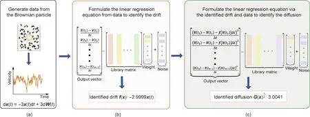
Fig. 1. Pipeline of the BISDE algorithm on the Langevin equation. (a) A Brownian particle (red dot) immersed in a fluid with its velocity satisfying the Langevin equation;(b, c) formulate the linear regression equation to identify the drift and diffusion from the space of candidate basis functions, respectively.

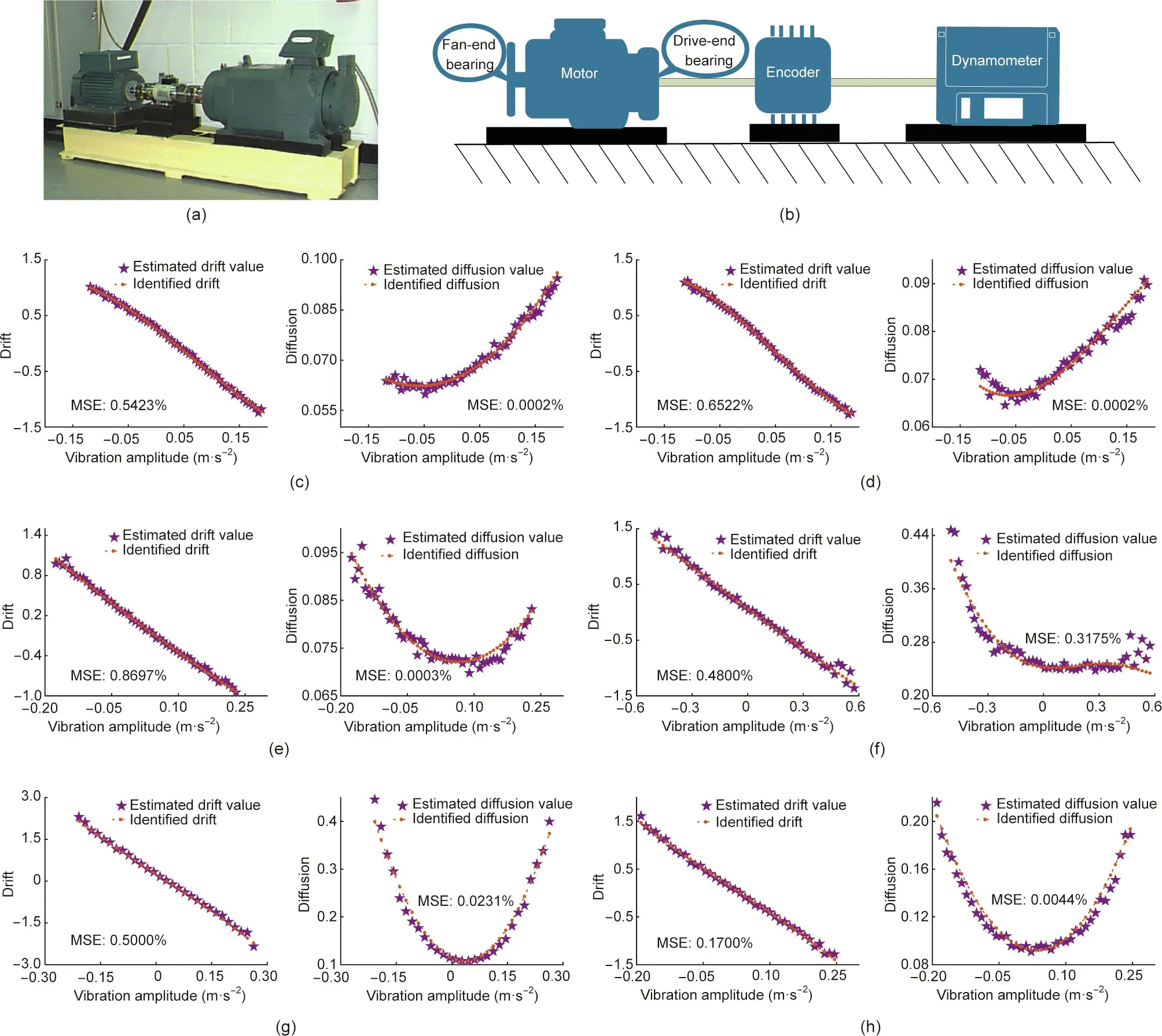
Fig. 2. Discovering the dynamics of normal and faulted fan-end bearings. (a) Bearing experimental platform of the CWRU dataset; (b) a cross-sectional view of the original test stand, consisting of a motor (left), a torque transducer/encoder (center), and a dynamometer (right); (c, d) identification results for NBs of 1 and 2 hp, respectively;(e,f)identification results for BF and IRF with the fault diameter of 7 mils,respectively(motor loads:1 hp);(g,h)identification results for BF and IRF with the fault diameter of 14 mils, respectively (motor loads: 1 hp).

We focus on the results of normal and faulted fan-end bearings of 1 hp herein;a more comprehensive comparison can be found in Section S3.2 in Appendix A.Because there is a sufficient amount of data, the binning operation can provide reasonable estimates for the drift and diffusion terms. Moreover, the estimates can be used as benchmarks to verify the identification results of BISDE.To illustrate that our method can reduce the required amount of data,BISDE only used about one-tenth of the dataset to discover the underlying dynamics. We present the comparison between the drift and diffusion estimates of the binning operation and the corresponding drift and diffusion identified by BISDE under different operating conditions in Figs. 2(c)–(h); the identified model’s performance was assessed using the MSE. This demonstrates that the identified drift and diffusion can accurately capture the dynamics of the bearing vibration signals. The identified models of NBs under different motor loads can aid operators or practitioners in conducting early diagnoses of faults to prevent disastrous consequences and reduce maintenance expenses.

3.3. Discovering the canonical stochastic models and applications

Finally,we applied the proposed BISDE algorithm to determine several canonical and real-world SDEs. The simulation models are based on common physical systems and stochastic processes(Sections S3.3–S3.5 in Appendix A).A two-dimensional simulation model is used to validate the power of the BISDE algorithm in identifying multidimensional SDEs from a limited amount of data.Realworld systems include stock price fluctuations, wind speeds, and oil prices (Sections S3.6–S3.8 in Appendix A). Enabling an identification framework for such stochastic dynamical systems can help practitioners improve system design and develop more efficient system management strategies for different scenarios. A more detailed illustration can be found below and in Section S3. Additionally, data and code implementations are available at https://github.com/HAIRLAB/BISDE.

Fig. 3 summarizes the simulated and real-world systems to be identified. Each category of three examples is marked with a specific background color. The first and fourth rows illustrate the simulated and real-world systems, respectively. The second row shows the simulated sample paths with colors denoting their probability density values, whereas the fifth row only shows real sample paths due to the lack of ground-truth information. The third and sixth rows assess the performance of the identified models.For simulated systems,we can compare the MSE between the data points generated by the real and identified drift/diffusion at measurements to assess its performance. We adopted Criteria 1, 2, and 3 to assess the identified models’ performance of realworld systems.

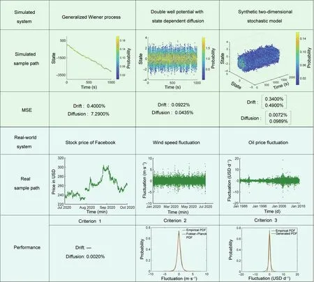
Fig.3. Summary of the BISDE algorithm applied to numerous examples. BISDE has been tested on three simulated systems, including a two-dimensional system, and three real-world systems, where each type is marked with a specific background color.

Comparison with state-of-the-art method: To demonstrate that BISDE can identify SDEs from relatively limited quantities of time-series data,we compared it with the state-of-the-art method in Ref. [17], which is referred to as SDE_SINDy hereinafter for convenience. Fig. 4 presents a visual comparison of BISDE and SDE_SINDy on the simulated systems. When the amount of data was relatively limited,SDE_SINDy failed to identify the underlying model structures for all cases, whereas BISDE yielded a nearperfect identification result.

Financial economics—stock prices: Stock prices are mutually influenced by many economic, financial, and political factors. The dynamics of stock prices can be considered a stochastic process because random noise introduces uncertainty when predicting future stock prices. In the 1970s, the weak-form efficient market hypothesis proposed by Eugene Fama, a recipient of the 2013 Nobel Prize in Economics, stated that future stock prices cannot be predicted by analyzing historical data [35]. Based on this hypothesis, stock prices are usually assumed to follow a Markov process. Lengthy historical data sequences are unhelpful in determining the dynamics of stock prices as these dynamics change over time [3]. Therefore, we collected the stock price data of Facebook every minute over three months from 1 July 2020 to 30 September 2020 (Figs. 5(a) and (b)).

After applying the proposed BISDE algorithm (Fig. 5(c)), the identified geometric Brownian motion model describing Facebook’s stock price behavior is shown in Fig.5(d).Geometric Brownian motion is the most widely accepted model for describing stock price behaviors [3], which is one of the assumptions used to derive the Black–Scholes–Merton formula to price European call and put options [36,37]. Surprisingly, the identified volatility(0.4039) almost coincides with the estimated volatility (0.4087)using the method suggested in Ref.[3],demonstrating the accuracy of the identified model. Compared with the one-year annual percentage yields (APY) provided by different banks (Fig. 5(e)), one can infer that the expected return on buying Facebook stock is several times the return on saving money in the given banks.Based on the identified model and one-year APY, investors can choose a strategy to balance the expected return and the uncertainty or risk of the stock to achieve better income (Figs. 5(f) and (g)). Overall,this application reveals that BISDE is a powerful tool for identifying the dynamics of stocks. The identified model can provide insights into stocks for investors and help determine price of stock options for stock exchanges [3].

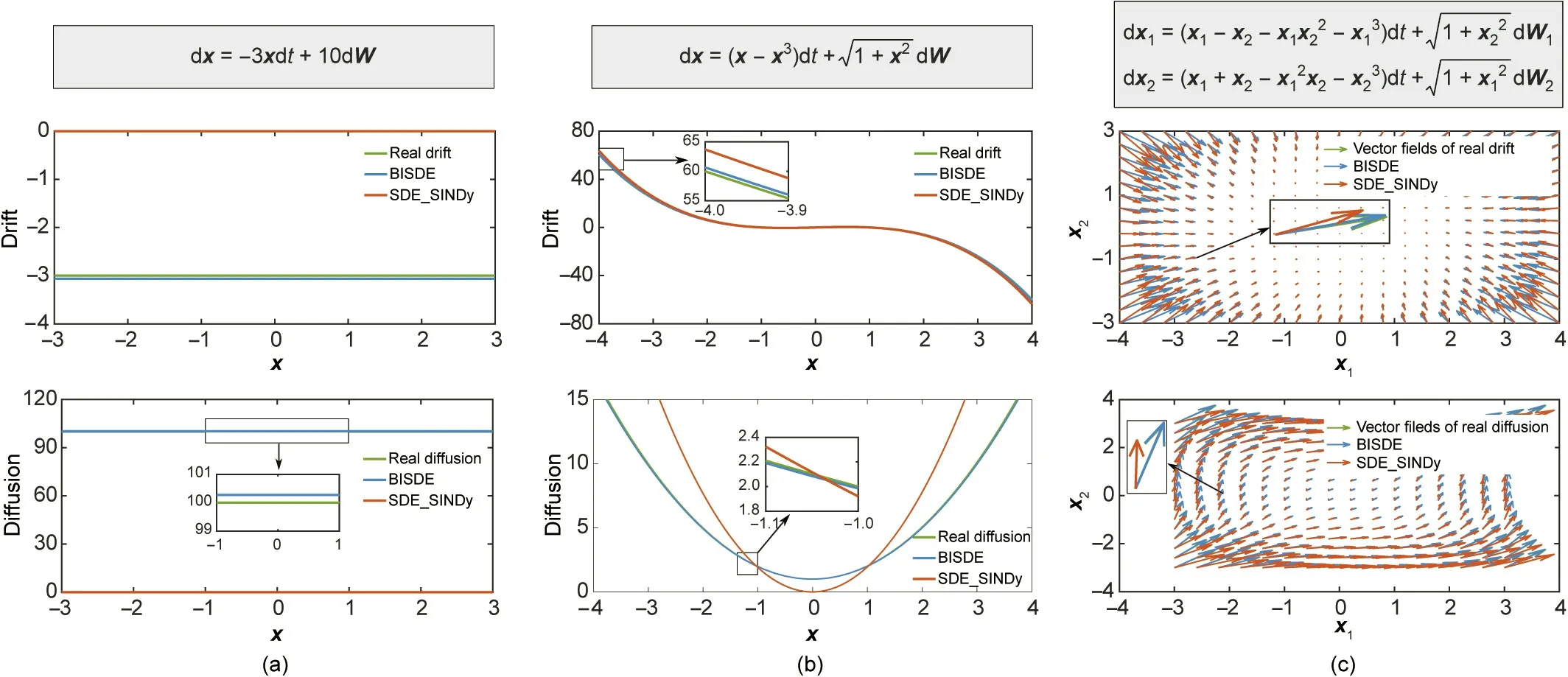
Fig.4. Comparison of BISDE and SDE_SINDy on the simulated systems.The identification results of BISDE and SDE_SINDy on(a)the generalized Winner process,(b)double well potential with state dependent diffusion, and (c) synthetic two-dimensional stochastic model.

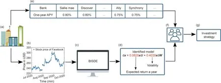
Fig. 5. Discovering the stock price behavior of Facebook. (a) Financial institutions (data acquisition); (b) stock price of Facebook over three months; (c) stock price data analyses; (d) identified SDE used to describe the stock price behavior of Facebook; (e) summary of the APY on one-year certificates of the deposit of different US banks in August 2020; (f) investors or technical analysts; (g) investment strategy made by investors by integrating investment information.

Power systems—wind speed fluctuations:As a widely distributed, sustainable, and renewable energy source, wind plays an important role in power grids across many countries. Globally,wind has accounted for approximately 5% of total power generation up to the end of 2020.Because wind speeds are uncontrollable and fluctuating under both spatial and temporal scales, the power production of a wind farm may vary from one minute to the next even when the total yearly production remains almost constant.Wind speed fluctuations affect the nominal power output, sometimes eroding power quality and reliability, as well as causing extreme gust and wind turbine fatigue loading[7,38,39].Therefore,determining the dynamics of wind speed fluctuations is essential for power production and load design to ensure the safety and economy of wind energy resources.

To illustrate the applicability of BISDE for this problem,we collected wind speed data for the first half of 2020 from Greta Point Cws, Wellington, New Zealand, located at 174.80574°E,41.30243°S, and 3 m above the mean sea level [40]. Wind speed fluctuations were obtained by calculating differences in wind speed data, resulting in the conversion of a non-stationary series(wind speed) to a stationary series (wind speed fluctuations). The identified model can be seen as the Ornstein–Uhlenbeck process with an added quadratic state-dependent term in the diffusion.Next,by solving the stationary Fokker–Planck equation,an analytical PDF for the identified model is derived. Its performance was verified by the high similarity between the analytic PDF and the empirical PDF generated by the measurements (Fig. 3). BISDE successfully identified an SDE to describe wind speed fluctuations. By embedding the identified model into wind turbine models,we can perform dynamic studies and thus maintain control of wind turbines [41,42].

Energy economies—oil price fluctuations:Despite the growing importance of renewable energy, oil continues to be the dominant resource in most countries. In contrast to almost all other commodities, oil has a considerable impact on the macroeconomy owing to its irreplaceability and high degree of liquidity in the international marketplace [43,44]. Oil price fluctuations cause significant losses or profits for both exporting and importing countries. Furthermore, oil price fluctuations may lead to inflation,increases in transportation costs,and changes in business policies,affecting not only industries but the daily lives of individuals and families. Because oil prices are affected by many independent and interrelated factors, an accurate model is challenging to formulate.

We applied the BISDE algorithm to resolve this challenging problem. To this end, we used crude oil prices collected from the US Energy Information Administration from the beginning of 1986 to the middle of 2017. First, we calculated the daily changes in oil prices. After determining the oil price fluctuations, we applied BISDE to discover the underlying dynamics. To illustrate the quality of the identified model, we generated a sample path based on the identified SDE with the same initial value as that of the real data. Then, we compared the empirical PDFs of the real and simulated data. The identified model yields a PDF very close to that of the real data in the high-probability region(Fig.3).Given current oil price fluctuations,the identified model can help predict the next fluctuation and address the corresponding uncertainties in terms of firms and policymakers, which are useful for avoiding unnecessary losses.

4. Discussion

This study provides a novel parametric algorithm called BISDE for the discovery of SDE-governed systems.This algorithm has several significant advantages. First, unlike non-parametric methods which cannot provide interpretable models [13], our algorithm identifies the model structures of the drift and diffusion terms to determine the underlying mechanisms of stochastic dynamical systems. Second, existing state-of-the-art data-driven algorithms project multidimensional systems to low-dimensional ones to reduce the required quantities of data [17,18]. In contrast, BISDE can directly discover original multidimensional systems with a limited amount of data. This capability was verified by the identification of a two-dimensional SDE and can be generalized naturally to higher-dimensional SDEs. Finally, although BISDE employs the Euler–Maruyama discretization method as in previous studies[10,13,14], we specified the limit conditions of the drift and diffusion terms, performed convergence analyses between the to-beidentified and real terms, and bridged non-parametric estimation with parametric identification. Overall, BISDE is a viable method for identifying the underlying dynamics of stochastic dynamical systems with relatively limited quantities of time-series data,and it possesses the potential to help researchers model natural phenomena and engineered systems perturbed by random noise from different sources.

Despite the advantages of BISDE, several questions remain.First, we note that prior knowledge is helpful in choosing basis functions, making the identification of model structures faster and more accurate. However, the lack of prior information makes it difficult to build libraries. To make matters potentially worse,true models may be approximated using polynomials, kernels,and other functional forms[22].There is also the question of establishing a verification method for non-stationary processes without knowing the exact model structures, because in many cases, we need to explore the intrinsic characteristics of state variables directly. Finally, two different SDEs may produce the same PDF(Section S4 in Appendix A), in which case they would possess the same statistical properties but involve two completely different mechanisms, which may mislead researchers.

Acknowledgments

This work was supported by the National Key Research and Development Program of China (2018YFB1701202), the National Natural Science Foundation of China (92167201 and 51975237),and the Fundamental Research Funds for the Central Universities,Huazhong University of Science and Technology (2021JYCXJJ028).

Authors’ contribution

Ye Yuan conceived of and supervised the project. Yasen Wang developed the algorithm and conducted experiments. All authors discussed the results and prepared and revised the manuscript accordingly.

Compliance with ethics guidelines

Yasen Wang, Huazhen Fang, Junyang Jin, Guijun Ma, Xin He,Xing Dai, Zuogong Yue, Cheng Cheng, Hai-Tao Zhang, Donglin Pu,Dongrui Wu, Ye Yuan, Jorge Gonçalves, Jürgen Kurths, and Han Ding declare that they have no conflict of interest or financial conflicts to disclose.

Appendix A. Supplementary data

Supplementary data to this article can be found online at https://doi.org/10.1016/j.eng.2022.02.007.