Data-Driven Model Falsification and Uncertainty Quantification for Fractured Reservoirs
Junling Fang, Bin Gong, Jef Caers*
a School of Earth Resources, China University of Geosciences, Wuhan 430074, China
b Key Laboratory of Tectonics and Petroleum Resources of the Ministry of Education, Wuhan 430074, China
c Department of Geological Sciences, Stanford University, Stanford 94305, USA
Keywords:Bayesian evidential learning Falsification Fractured reservoir Random forest Approximate Bayesian computation
A B S T R A C T Many properties of natural fractures are uncertain,such as their spatial distribution,petrophysical properties,and fluid flow performance.Bayesian theorem provides a framework to quantify the uncertainty in geological modeling and flow simulation, and hence to support reservoir performance predictions. The application of Bayesian methods to fractured reservoirs has mostly been limited to synthetic cases. In field applications,however,one of the main problems is that the Bayesian prior is falsified,because it fails to predict past reservoir production data. In this paper, we show how a global sensitivity analysis (GSA)can be used to identify why the prior is falsified.We then employ an approximate Bayesian computation(ABC) method combined with a tree-based surrogate model to match the production history. We apply these two approaches to a complex fractured oil and gas reservoir where all uncertainties are jointly considered,including the petrophysical properties,rock physics properties,fluid properties,discrete fracture parameters, and dynamics of pressure and transmissibility. We successfully identify several reasons for the falsification.The results show that the methods we propose are effective in quantifying uncertainty in the modeling and flow simulation of a fractured reservoir. The uncertainties of key parameters, such as fracture aperture and fault conductivity, are reduced.
1. Introduction
Naturally fractured reservoirs constitute a significant portion of the world’s remaining oil and gas reserves[1,2].Although the existence of fractures enhances the fluid storage and flow capacity[3,4], it also brings significant challenges to oilfield development[1].In reservoir modeling and simulation,many fracture properties are uncertain, such as the discrete fracture network (DFN) parameters [5,6], permeability anisotropy [2], relative permeability and wettability [7,8], and dependence of fracture permeability on reservoir pressure [9,10]. Thus, uncertainty quantification plays a critical role in mitigating decision-making risk in fractured reservoir development.
The information gained from different sources, such as threedimensional (3D) seismic surveying [11-14], fracture field outcrops [2,15-17], borehole imaging logging [18,19], and laboratory experiment data [10], contributes to reducing the uncertainty in static reservoir modeling and dynamic flow simulation.
The uncertainty quantification of reservoir prediction is often performed by generating multiple models constrained by the production history [20,21]—namely, posterior realizations. Bayesian theorem is a commonly used framework to generate (posterior)models[22],based on a stated prior and a likelihood model.When used on fracture properties, a prior model makes it possible to impose important geological characteristics[23,24]generated from Monte Carlosimulations onto the model.In the Monte Carlo method,uncertain variables are randomly sampled.The Markov chain Monte Carlo(McMC)method is introduced to target the distribution from which we want to sample. Recently, the McMC method has been increasingly used in history matching and uncertainty quantification [21,25]. McMC generates a dependent chain of models that makes it possible to estimate and sample the posterior distribution.In each iteration of the Markov chain,an acceptance rule is used to decide whether to accept the proposed model or retain the old model. Several modified McMC approaches have been developed to enhance the performance of the McMC method;examples include hybrid McMC[26],mode jumping McMC[27],and parallel interacting McMC[28],which deal with low acceptance,multi-mode posterior,and high-dimensional issues arising in practical applications.
The efficiency of McMC methods is limited because the realizations are sequentially generated. Ensemble methods—such as the ensemble Kalman filter (EnKF) [29-31], ensemble smoother (ES)[32,33],iterative EnKF[34],and ensemble smoother with multiple data assimilation (ES-MDA) [35]—have recently gained attention for quantifying uncertainty and history matching.EnKF is a Monte Carlo method that implements a covariance-based Bayesian updating scheme for data assimilation[31].The prior model parameters and production data are jointly updated through assimilation by the observation data under the primary assumptions of linear system dynamics and multivariate Gaussian distribution of the model parameters.The ES method is used to avoid rerunning the simulation as the parameters are updated, while the iterative EnKF extends the assumption of the EnKF to be applicable when the relationship between the data and model parameters is highly nonlinear. The ES-MDA improves the ES method by introducing an inflated error covariance matrix.
More recently, direct forecasting [24,36,37] and data-space inversion[38,39]have been introduced to evaluate the uncertainty of future reservoir performance prediction without generating posterior reservoir models. Instead, direct forecasting establishes a statistical model between the (historical) data and the target(future prediction).The posterior prediction distribution is directly estimated from the observations. Data-space inversion treats production data as random variables. The posterior data variable distribution is sampled through a data-space randomized maximum likelihood method.
However, these methods do not address a case in which the prior distribution is falsified [40]. Falsification simply means that the stated model can never predict the historical data, no matter how many realizations are generated.Bayesian evidential learning(BEL) [41] offers a protocol for uncertainty quantification that includes falsification. It is increasingly used to quantify the uncertainty in oil and gas [24], groundwater [42], and geothermal [23]applications. Rather than being a method, BEL is a protocol of how existing methods can be applied to solve field case problems.The advantage of BEL is that it can handle any distribution of the prior and any sensitivity analysis methods,which makes it applicable to quantify the uncertainty of complex problems in practice.
Many uncertainty quantification processes are time-consuming,as they usually require the generation of thousands to tens of thousands of model samples from geological modeling and forward simulation. In fractured reservoirs, significant computational cost must be considered in order to capture the detailed fluid flow in fractures using an unstructured grid explicitly or a refined structured grid. This challenge makes it attractive to build surrogate models (also known as proxy models) as less computationally expensive alternatives for practical fractured reservoirs.Many surrogate models have been developed for history matching and uncertainty quantification, such as polynomial models, kriging models,splines proxy models with space-filling designs,and more widely used response surface proxy models [43-45]. More recently, the use of tree-based regression, such as random forest models [46] and stochastic gradient boosting [47], for sensitivity analysis and history matching has obtained increased attention.
Many studies on and methods for uncertainty quantification use synthetic cases(e.g.,Ref.[39]),in which the prior uncertainties are manually designed, and the observed data are selected from the simulated results.This simplification bypasses the falsification issue because the selected‘‘truth”from the simulation is always in the population of prior data, indicating that the probability of the observation in the prior is prominent enough. In real cases, the prior model uncertainty—as determined through careful geological, geophysical, and engineering analysis—is often unable to predict the actual observations, meaning that the prior model is falsified[40].The prior model may be falsified for various reasons:the parameter uncertainty may be too narrow or taken to be deterministic,the physical model used may be incorrect,or any combination of both may occur [23,48].
Falsification problems are often reported in prior-based techniques [24,49]. However, a systematic approach—namely, defalsification—is needed to diagnose the prior problem and adjust it to become non-falsified.The first main contribution of this paper is that we present a systematic approach that indicates what is wrong in the prior model when the prior model is falsified. We combine global sensitivity analysis (GSA), dimension reduction,and Monte Carlo techniques to identify the problem. The second contribution is that we employ an approximate Bayesian computation (ABC) method combined with a random-forest-based surrogate model trained on the non-falsified prior to match the production history. Finally, we apply this method to a complex fractured reservoir for which all uncertainties are jointly considered,including petrophysical properties,rock physics,fluid properties, and fracture properties.
The field case is a naturally fractured metamorphic reservoir located at the Bohai basin in China, where decision-making under uncertainty is needed in order to plan additional wells.The uncertainty components include fracture density,fracture aperture,permeability at the well location and spatial distribution, relative permeability, and fault transmissibility. The problem is how to evaluate and, more importantly, how to reduce the uncertainty of the reservoir model based on the measured data (i.e., well logging and seismic data)and the historical data(i.e.,production rates and pressure).
2. Case study
2.1. Bayesian evidential learning for field cases
BEL is a comprehensive framework for uncertainty quantification and inversion [41]. Rather than being a method, BEL is a protocol based on Bayesian reasoning with priors. It uses a GSA to suggest effective inverse methods (i.e., history matching) for the case at hand, and it uses observations (i.e., the production history data in this study)as evidence to infer model hypotheses by learning from the prior distribution [24]. In general, BEL consists of six stages [23]:
(1) Formulation of the decision problem and definition of the prediction variables;
(2) Statement of the prior uncertainty model;
(3) Monte Carlo simulation and falsification of the prior uncertainty model;
(4) GSA of the data and prediction variables;
(5) Uncertainty reduction with the data;
(6) Posterior falsification and decision-making.
This work aims to quantify uncertainty in reservoir modeling and simulation processes; it corresponds to Stages 2-5 in the framework.
2.2. Geological settings and production history
The study area is an offshore, naturally fractured burial-hill reservoir located in China. The reservoir consists of metamorphic rocks, which are impermeable. Before being buried to the subsurface, the top of the reservoir was weathered, forming a capacity for storage and fluid mobility.Natural fractures are caused by both weathering and tectonic movement. Five producers are drilled in the upper area of the reservoir, surrounded by four injectors in the relatively lower part of the reservoir (Fig. S1(a) in Appendix A). There are two exploration wells are drilled, but not brought to producing or injecting.
The fluids in the reservoir are oil and water, which are separated by a constant oil-water contact (WOC) near-1880 m(Fig. S1(b) in Appendix A). The reservoir started to produce oil in September 2015. The production history data of the five production wells are collected (Fig. S2 in Appendix A). The observation data are the oil production rate (OPR), gas production rate (GPR)for all the production wells, and the bottom hole pressure (BHP)for the production wells P1, P2, and P3. No water production occurred for any of the production wells until March 2019.
2.3. Reservoir modeling data and prior uncertainty elicitation
Uncertainties remain in many aspects of static modeling and flow simulation,such as structure modeling,petrophysical modeling, fluid modeling, and rock physics modeling. In this section, we describe the information available for characterizing the reservoir and the sources of uncertainty throughout the modeling and simulation processes.The quantified uncertainty parameters and their distribution are listed in Table 1, and the whole modeling workflow is shown in Fig. 1.
2.3.1. Structural uncertainty
The reservoir is divided into three vertical zones (Fig. S3(a) in Appendix A). The ratio of the reservoir to non-reservoir decreases because the weathering degree decreases from top to bottom.Forty-six faults (Fig. S3(b) in Appendix A) are interpreted from the 3D seismic ant tracking attribute (Fig. S4 in Appendix A). The position of all the faults is deterministic,while the fault conductivity remains uncertain because the fault conductivity is difficult to measure in the reservoir. Here, we simplify the fault conductivity uncertainty as two scenarios: fully sealed and fully opened.
2.3.2. Petrophysical property uncertainty
Petrophysical properties, such as porosity and permeability,have uncertainties. In this case, matrix porosity is measured from well logs. Seismic acoustic impedance (Fig. S4 in Appendix A) is measured to indicate the spatial variation of the porosity. We apply co-SGS to simulate the 3D property distribution with log interpretations as ‘‘hard” data and the seismic attribute as ‘‘soft”data. In the matrix property modeling process, the uncertain modeling parameter includes variogram parameters, and the correlation coefficient of the seismic attribute to the borehole properties. Matrix permeability is not measured at well locations.Thus, we provide a prior depending on past experience. The spatial distribution of the matrix permeability is constrained by the porosity.
2.3.3. Uncertainty in fracture properties
Fractures may have a considerable impact on fluid flow. The four existing wells (two production wells and two exploration wells) directly measure the fracture information using image logging, including fracture density and orientation. The spatial variation of the fracture density can be indicated by the seismic azimuthal anisotropy (Fig. S4 in Appendix A). We use co-sequential Gaussian simulation (co-SGS) to simulate the 3D fracture density model under the constraint of a seismic azimuthal anisotropy cube. Several modeling parameters are uncertain, such as the variogram and correlation coefficient with the seismic attribute. A stochastic DFN model is then built using the fracturedensity, fracture orientation, fracture length distribution, fracture aperture, and so forth. The fracture orientation is constrained by the trend of the fault lines, while the deviation of the fracture orientation to the fault line is uncertain. The DFN model is then upscaled to continuous grid properties using the Oda method[50] to reduce the computational complexity in the fluid flow simulation.
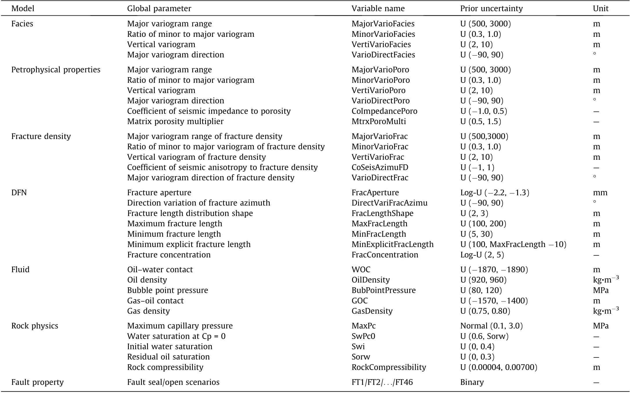
Table 1 Uncertainty parameters and their distribution.
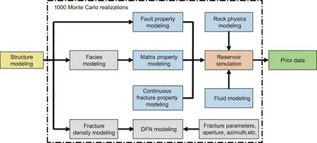
Fig. 1. Reservoir modeling and reservoir simulation workflow.
2.3.4. Rock and fluid property uncertainties
Fractures make it difficult to obtain rock physics measurements and interactions between fluids and rocks. In this case, no direct measurement—such as rock compressibility, relative permeability curves, initial water saturation, or capillary pressure—is available for the reservoir. Thus, we refer to previous research [8,51] and similar reservoirs to define the rock physical properties and uncertainty ranges.The pressure-volume-temperature(PVT)properties,including the bubble point pressure,oil and gas density,and other fluid distribution parameters, such as gas-oil contact (GOC), and oil-water contact (WOC), are treated as uncertain by introducing a range around a reference (base-case) value provided by the oil company.
2.3.5. Table of all prior uncertainties
Bayesian model-based uncertainty quantification requires a prior statement of the model parameterization and a probability distribution for each parameter. In the analysis of uncertainty sources in the previous sections, we observe that many aspects of properties are uncertain, including petrophysical properties,fluid storage, PVT, rock physics, and the spatial heterogeneity caused by the different scales of fractures. On the one hand, we try to consider every possible uncertain parameter in the entire modeling and simulation process to avoid missing important parameters.On the other hand,we need to balance the model complexity and computational demand to address multiple uncertainties affordably. Detailed names and distributions of the uncertain parameters are listed in Table 1.
2.4. Static modeling, flow simulation, and Monte Carlo simulation
Because physics-based models for subsurface systems are high-dimensional and nonlinear, Monte Carlo simulation is needed. Each variable specified in the prior model is sampled according to its probability distribution to generate a singlemodel realization via Monte Carlo simulation. We apply a dual-porosity dual-permeability simulation as a forward model to compute the production data as a response to the variation of uncertain parameters. Two commercial software, PETREL and ECLIPSE E100,are used to do static modeling and reservoir simulation,respectively.The forward model function can be formalized as follows:

where gdis a deterministic function that maps a model to data variable d, the simulated production data. mmatrixis a matrix model;mfracis a fracture model; mfaultis a fault model; mfluidis a fluid model,including fluid contacts and PVTs;and mrockis a rock physics model, including the rock compressibility, capillary pressure, and relative permeability.
The entire workflow of geological modeling and reservoir simulation is shown in Fig. 1. We perform Monte Carlo sampling of all uncertain parameters from the distribution of Table 1; 1000 models (Fig. S5 in Appendix A) and simulations are generated.
Fig. 2 shows the simulated production data compared with the production history.It can be seen that,for some of the production curves,the prior appears to cover the observations,such as the gas rate of wells P1, P3, P4, and P5. This is not the case for the BHP curves of well P3.The BHP of P1 and the gas rate of P2 have a certain degree of coverage but have a different trend in time. These results indicate that the prior is not adequate,even when considering many aspects of uncertainty.
In the next section, we develop a systematic approach to identify what is wrong with the prior and, more importantly, how we can correct the prior when it is falsified.
3. Methodology
3.1. Falsification in Bayesian evidential learning
Once the forward functions are established, it is necessary to check whether or not the defined prior model is falsified.A falsified prior means that the prior statement is not informative to cover the observation.As a result,the posterior calculation will be unsuccessful. In probabilistic approaches, it is common to attempt to prove that the prior model is incorrect rather than proving it is correct (i.e., to reject the null hypothesis of ‘‘the prior model predicts the data”).If the prior model cannot be falsified,then the assumptions it made have been strengthened but are not necessarily proven to be correct. The falsification process can be achieved by verifying: ①that the model reproduced known physical variation in the system,or ②that the model can predict observed data[23].The latter does not entail matching historical data (i.e., observed data,dobs),but rather indicates that the probability of the observed data within the population of generated data responses using Eq.(1)is not zero.This falsification process has been used in many previous studies [25,42,52]. Developing the prior model is typically iterative, meaning that the first choice of a prior model tends to be falsified.Depending on the reason the prior model was falsified,the prior model may need to be adjusted by increasing ①the model complexity, ②the parameter uncertainty, or ③both.
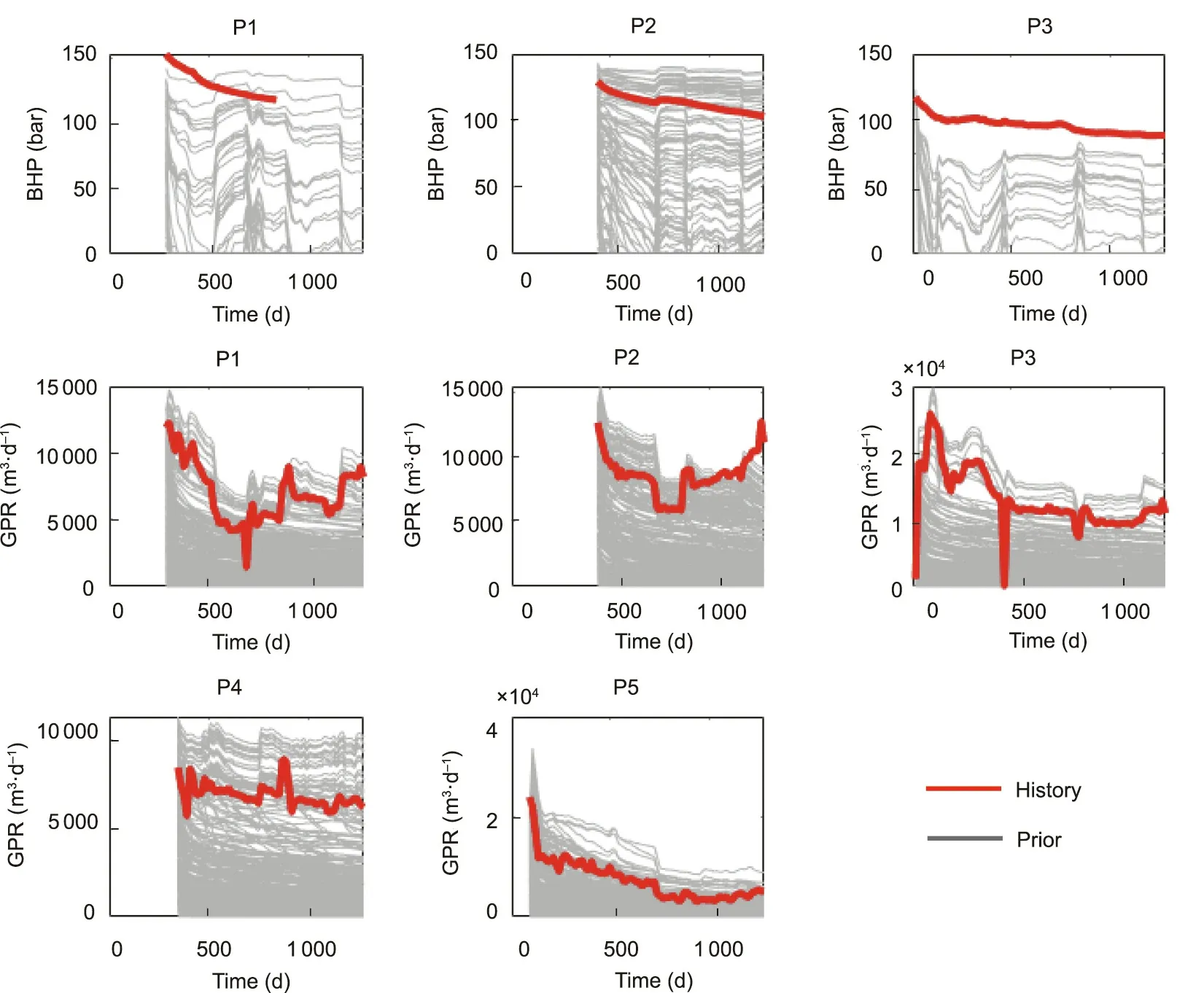
Fig. 2. Simulation data using the prior defined in Table 1.
When the data variable is of low dimension,falsification detection is straightforward by means of visual inspection.In this study,the data variable is high-dimensional,which means that a systematic method is required. Mahalanobis-based methods have gained attention for falsification detection. Yin et al. [24] used a robust Mahalanobis distance (RMD) method to detect the prior with a multi-Gaussian distribution. In the application of field cases, the simulated production data may not be Gaussian. Alfonza and Oliver [48] used an approximation of the Mahalanobis distance between the observation and the ensemble of simulations to diagnose the prior model parameters. Their method can be used for both Gaussian and non-Gaussian data,as well as large models with large amounts of data. However, their method focuses on how many samples are accepted to improve the prior model.The results do not give a straightforward criterion of whether or not the prior model is falsified. A one-class support vector machine (SVM) is a popular outlier detection method[41,53], in which a minimal volume hypersphere around the samples in data space is fit. Any observation that falls outside of the hypersphere is classified as inconsistent with the prior. Using kernels, a one-class SVM provides a powerful tool for detecting outliers in high dimensions and with nonlinear decision boundaries. We employ a one-class SVM as a falsification method to diagnose the prior model.
3.2. Global sensitivity analysis
Another way of analyzing Monte Carlo simulations is by means of a GSA, which investigates what model parameters (or a combination thereof)influence the response(e.g.,simulated production).GSA methods are based on Monte Carlo sampling, in which all parameters are varied jointly [54]. In this study, we perform a GSA using the distance-based generalized sensitivity analysis(DGSA) method [55,56]. DGSA is a regionalized GSA method [57]that reduces the number of samples into a small number of classes.The distances between the prior cumulative distribution functions(CDFs) and the class-conditional CDFs are then calculated to measure the sensitivity. One advantage of DGSA is that it supports all types of input parameter distributions, such as continuous, discrete, and scenario-based distributions. Another advantage of DGSA is that it accounts for the possible high-dimensional responses of the computer models[41],which is typically the case in subsurface systems.
We employ DGSA to assist in the de-falsification of the prior in two aspects.The first aspect is the adjustment of the current prior model parameters.DGSA simplifies the de-falsification by filtering out the non-sensitive parameters by reducing the model complexity. Another aspect is that prior model complexity may be increased by adding new uncertain parameters. DGSA can examine the effectiveness of the new model parameters. In the application, we will show how DGSA can be used to identify the problem when the prior model is falsified.
3.3. Uncertainty quantification with data
If the prior is not falsified, a proper Bayesian uncertainty quantification can proceed. The full Bayesian approach estimates a likelihood function P(d|m) occurring under the prior distribution P(m). The posterior distribution of the model P(m|d) is then calculated via the following formula:

However,it is computationally expensive—or completely infeasible—to evaluate the likelihood in real cases with high-dimensional and different distribution types of parameters[58].Here,we employ an ABC method to generate the posterior distribution of the variables[58,59]. ABC methods are rooted in rejection sampling. An ABC approximates the likelihood function by comparing simulated data with the observed data.In ABC methods,the model m is accepted if its simulation data gd(m )is close to the observed data dobs.Thus,this method bypasses exact likelihood calculations[60].The probability of generating accepted models with a small distance to the observed data decreases as the dimensionality of the data increases.Summary statistics,which are values calculated from the data to represent the maximum amount of information in the simplest possible form,are introduced into the ABC method to replace the data. This method accepts the samples if the summary statistics of the simulated dataset are within a distance ε from the summary statistics of the observed dataset. The distribution of the accepted samples is an approximation of the posterior given by the following:

where I(d(gd(m),dobs)<ε)is a summary statistic that defines a window size ε, defining the acceptance region.
It is essential to highlight that, unless data d is sufficient, the approximation error does not vanish as ε →0 [58,60].On the other hand,the acceptance rate decreases as the dimension of data variable d increases.We should then increase ε,which leads to an approximationoflowerquality.Based onthelimitations,wemust:①generateas many as realizations of model m as possible and simulate model m to data d;and ②reduce the dimension of data variable d.
Since DFN modeling and simulation for a field case with millions of grid cells are very time-consuming,it is impractical to generate as many realizations as are required by the ABC method,which may be tens of thousands. Thus, a surrogate model is needed, which will be explained in the next section.
3.4. Surrogate model
3.4.1. Tree-based regression
We perform a tree-based regression [61] surrogate model to replace the time-consuming static and forward modeling. Using a tree-like topology,the tree-based method is based on a binary partition of the input space and model y employing a constant in the partitioned region. The model output is piecewise discontinuous,which can be formulated as follows:

where cmis a constant;Rmis partitioned region;I(x)is a linear combination of discrete indicator functions over M regions. The advantage of the regression tree is that it works for both continuous and categorical input variables, which is often the case in geological issues. However, due to the piecewise nature, the regression tree method trades off regression accuracy. Its predictive precision is less than most other methods [62].
3.4.2. Ensemble trees
‘‘Boosting”[63]and‘‘bagging”[64]are two ways to improve the prediction performance of a tree-based regression via an ensemble of trees.The boosting regression tree method uses the outcomes of weaker estimators to enhance the prediction performance by combining the strengths of each weak classifier [65,66]. The trees of boosting method are generated sequentially.In each step, the tree estimator is trained with early estimators,fitting simple models to the data and then analyzing the data for errors. The weights of samples with more significant errors are then increased. The final estimator takes a weighted combination of the sequence of estimators. Gradient boosting is an extension of the boosting method; it combines the gradient descent algorithm to optimize the differentiable loss function. The new tree of each generation attempts to recover the loss between the actual and predicted values [65].
Bagging (bootstrap) aggregation [64] with trees creates several subsets of data randomly chosen with replacements from training samples.The tree estimators are trained independently using each subset of the data. The final estimator is created by averaging all the estimators generated from different trees with these bootstrap samples. The random forest [67] method is an extension of bagging.In addition to selecting a random subset of data, it randomly selects the input features instead of using all features to grow trees.This extension handles missing values, maintains accuracy for missing data, and handles higher dimensionality data very well.
4. De-falsification and uncertainty quantification: a case study
4.1. Falsification identification
We now return to the case study and follow the sequence of the BEL protocol. We have stated the prior uncertainty and performed a Monte Carlo simulation; hence, the next step is falsification detection.We map the simulated data and observed data in lower dimensions, and then perform an outlier detection test on the lower-dimensional space to perform falsification detection. Here,we use principal component analysis (PCA) for dimension reduction.Fig.3 shows the principal component(PC)score plots for different responses and wells.
As shown in Fig. 3, some observations (red dots) are far away from the simulation data points(gray dots),such as the BHP of well P3 and the gas rate of well P2. Some observations are close to the simulation points but do not have enough coverage, such as the BHP of well P1, the gas rate of well P1, and the gas rate of well P3. The BHP of well P2 does not seem to be falsified, because the observation dot is inside the prior dots in the PC1 and PC2 plots.However,it is falsified in the higher dimension.This can be viewed in the PC2 and PC3 plot (Fig. 4).
Thus,the prior we defined is falsified—that is,it is proven incorrect. We need a systematic method to identify the problem with the prior. Any revision would need to increase the uncertainty,add complexity, or perform some combination of the two. Simple ad hoc modifications such as multipliers on parameters are non-Bayesian[40].Instead,we will formulate the problem as a hypothesis test.We will make revisions to the prior,state this as a hypothesis, and then attempt to reject this as a hypothesis.
4.2. Hypothesis 1: incorrect distribution of current uncertain parameters
To identify what the problem is with the prior, we perform DGSA to conduct a sensitivity analysis. The result (Fig. 5) shows that the fracture aperture is the most sensitive parameter. The PCA plot (Fig. 4) shows that the points closer to the observation are more likely to have a larger fracture aperture value. Those two features indicate that the fracture aperture distribution might be too narrow. Thus, we increase the upper limit of the fracture aperture distribution from -1.3 to -0.2, and the lower limit remains as -2.2.
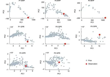
Fig. 3. PCA plot of the data for each production well and data type. Gray points are the simulations, and red dots are the actual field observations.
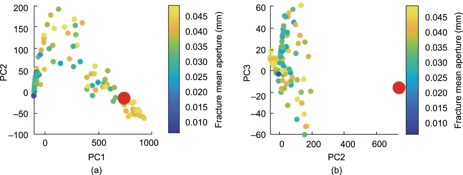
Fig.4. PCA plot of P2 BHP data.(a)PC1 and PC2 plot;(b)PC2 and PC3 plot.The color of the dots represents the fracture aperture value.Red dots are the PCs of observations,while other dots are the PCs of the prior data.
After increasing the range of the fracture aperture of the prior,we redo the Monte Carlo and reservoir simulation to generate the prior data(Fig.S6 in Appendix A).Fig.6 shows a comparison of the prior data of Hypothesis 1(blue dots)and the initial prior(gray dots).It can be seen that the data points of Hypothesis 1 have more coverage of the observation.This evidence indicates that Hypothesis 1 is not wrong. However, the prior is still falsified, even though the data has more coverage of the observation than the initial prior.As shown in Fig.6,the observation points of the gas rate of well P2 and the BHP of well P1 are still outside of the simulation points.Thus,we should propose new hypotheses to figure out the prior problems.
4.3. Hypothesis 2: add model complexity—dynamic transmissibility
As shown in Fig. 2, the BHP history curve of well P1 continuously decreases during the production. However, the simulated curves are flatter,which means that the borehole has a much more fluid supply in the simulation than in reality.One potential reason is that the permeability is pressure-dependent—that is,the permeability is dynamically changing with the reservoir pressure. This phenomenon has been investigated by several studies [9,10] for fractured reservoirs. We missed this mechanism in the definition of the previous prior. Chen et al. [10] reported a power-law relationship of the fracture permeability changing with reservoir pressure drawdown. The function is as follows:
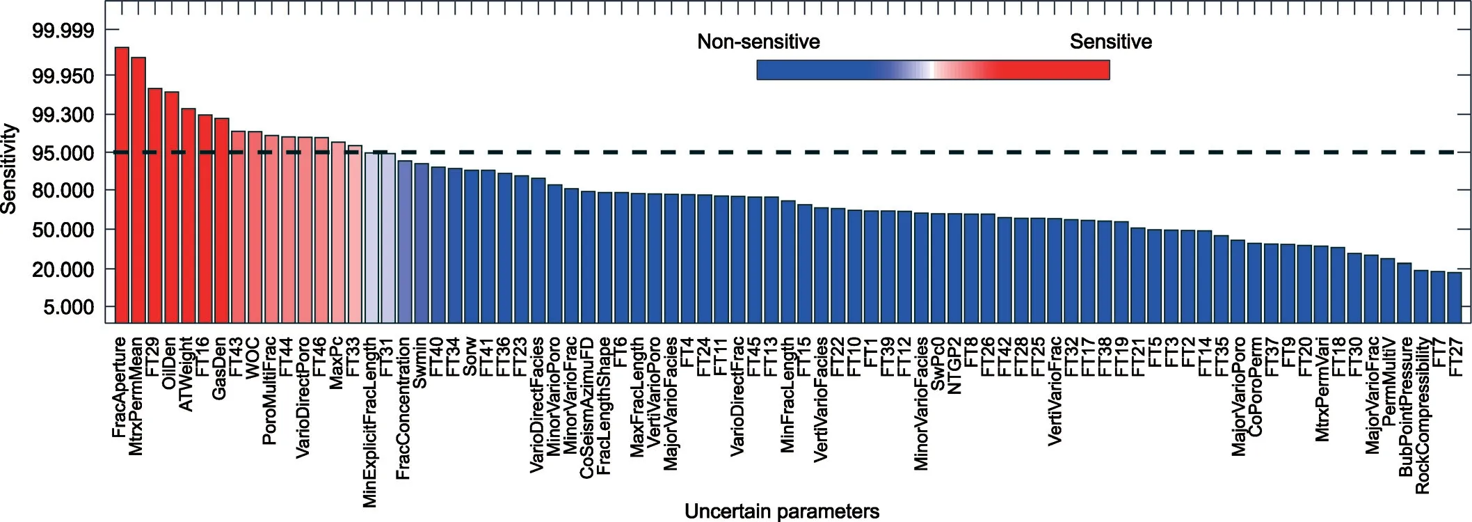
Fig. 5. Sensitivity analysis of the uncertain parameters for the BHP data of well P2.
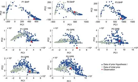
Fig. 6. Comparison of the data with Hypothesis 1 to the data of the initial prior.

where p0is the reference pressure,p is the reservoir pressure, k0is the fracture permeability at p0,cfis the rock compressibility,ν is the Poisson’s ratio, and αbis the Biot coefficient.

When the dynamic transmissibility multiplier is added to the model, the Monte Carlo simulation results have a larger observation coverage both on simulation curves (Fig. S8 in Appendix A)and PCA plots (Fig. S9 in Appendix A). The results of DGSA shows that the dynamic transmissibility multiplier is sensitive to the simulation data(Fig.S10 in Appendix A).These evidences indicate that the hypothesis is not wrong; it should be considered in the prior model. However, closer inspection of the gas rate points of well P2 (Fig. S9 in Appendix A) shows that the observation is still outside of the prior data points.The production curves in Fig.S9 show that the production history of the gas rate in P2 increases after the year 2018,while the simulated curves do not have this feature.The BHP observation of well P2 decreases during the production history. This shows that the model we built is still not complex enough to reflect all the features remaining in the production his-tory.The possible reason for this phenomenon is that the pressure supply is insufficient, leading to degasification in the area of wells P1 and P2. This is reasonable, because the peak of the reservoir is located in this area.

Table 2 Modification of the prior in Hypothesis 2 and Hypothesis 3.
4.4. Hypothesis 3: Add model complexity—decrease the pressure supply of the producers
Pressure supply comes from two aspects: bottom water and injectors. We introduce two additional uncertain parameters—the fracture aperture decreasing degree from top to bottom(Fig. 7(a)) and the pore volume multiplier of the bottom zone(Fig. 7(b))—to represent the pressure supply uncertainty from the bottom water. In the original fault network (Fig. 7(c)), it can be seen that the production wells P1 and P2 are not fully separated by the faults from the nearby injection wells, INJ1 and INJ2. This means that, even though the faults are fully sealed, there are still some connections between the producers and injectors.This might be a reason for the abundant pressure supply of wells P1 and P2.Here, we define a variable that represents whether or not we use a modified fault network. The added parameters are listed in Table 2, and the fault modification strategy is shown in Fig. 7(c).
We then perform Monte Carlo simulation to generate the prior data. The simulation results (Fig. S11 in Appendix A) show that some of the BHP curves behave more consistently with the field observations for wells P1 and P2. More importantly, some of the gas rate curves for well P2 start to increase after 2018, which was not captured in the previous priors. The prior data points of PC1 and PC2 have good coverage of the observation (Fig. S12 in Appendix A).The DGSA result(Fig.S13 in Appendix A)also reveals that the Hypothesis 3 should be included in the prior.
Thus far,we have proceeded with a visual inspection of the lowdimensional PC score plots.Now,we include all PC dimensions and use a systematic method to detect falsification. We employ a oneclass SVM, an outlier detection method, to perform falsification detection. The logic is that, if the observations are an outlier relative to the simulated observations, then the prior is falsified. We employ a one-class SVM rather than the Mahalanobis distancebased method because the data distribution is not Gaussian(Fig. 8(a)).
In a one-class SVM,all the simulation data are considered to be training samples for training a classification model. Then the observation score is calculated using the trained model. An observation with a negative score is considered to be an outlier, which means that the prior is falsified. Fig. 8(b) shows that the observation score is still positive when 10 PCs containing more than 99%of the information are included in the training data. This reveals that the prior is not falsified.
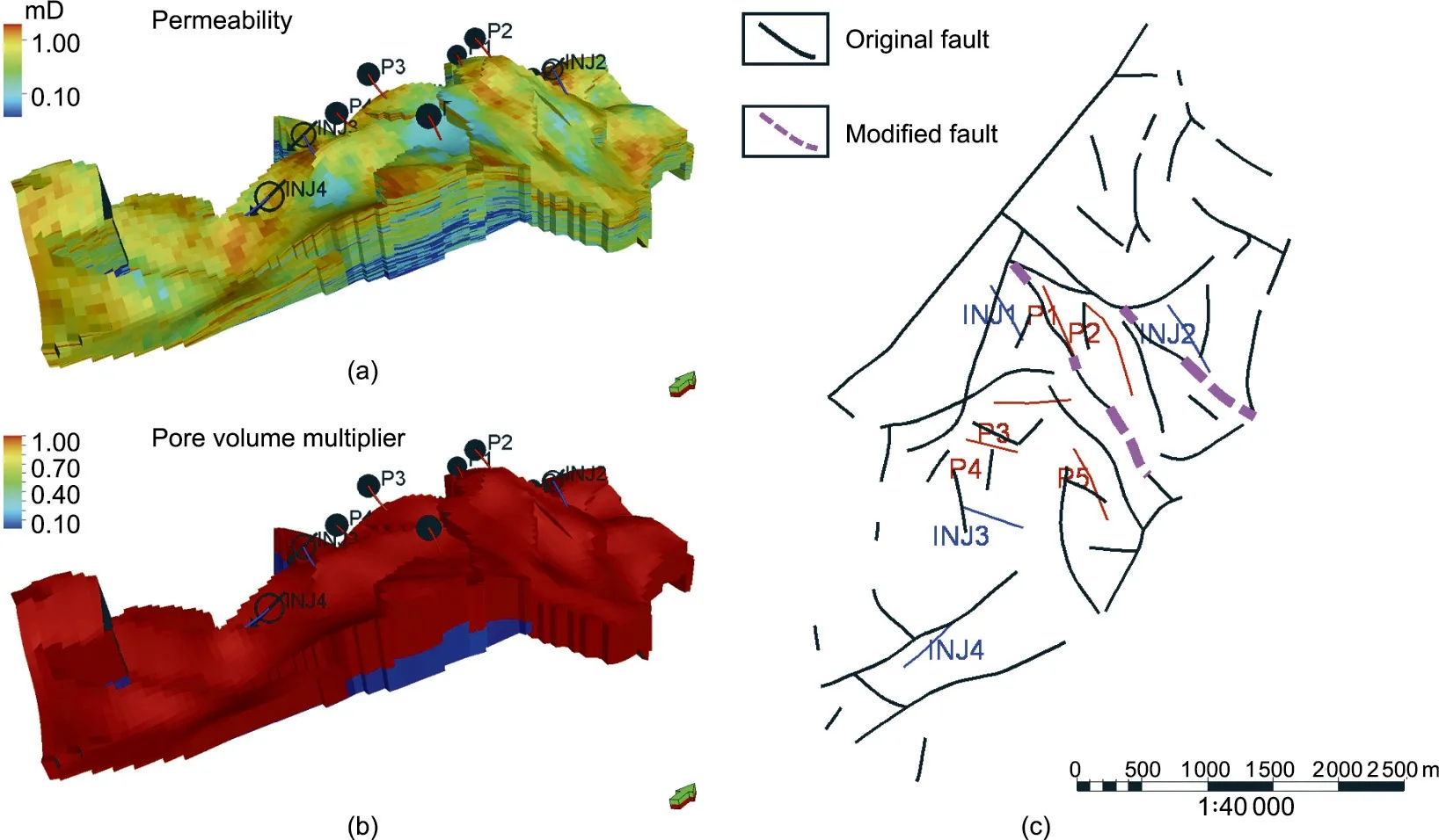
Fig. 7. Model modification in Hypothesis 3. (a) One realization of permeability, considering the decreasing degree of the fracture aperture from top to bottom; (b) one realization of a pore volume multiplier for Zone 3; (c) fault modification. INJ: injector. mD: millidarcy.
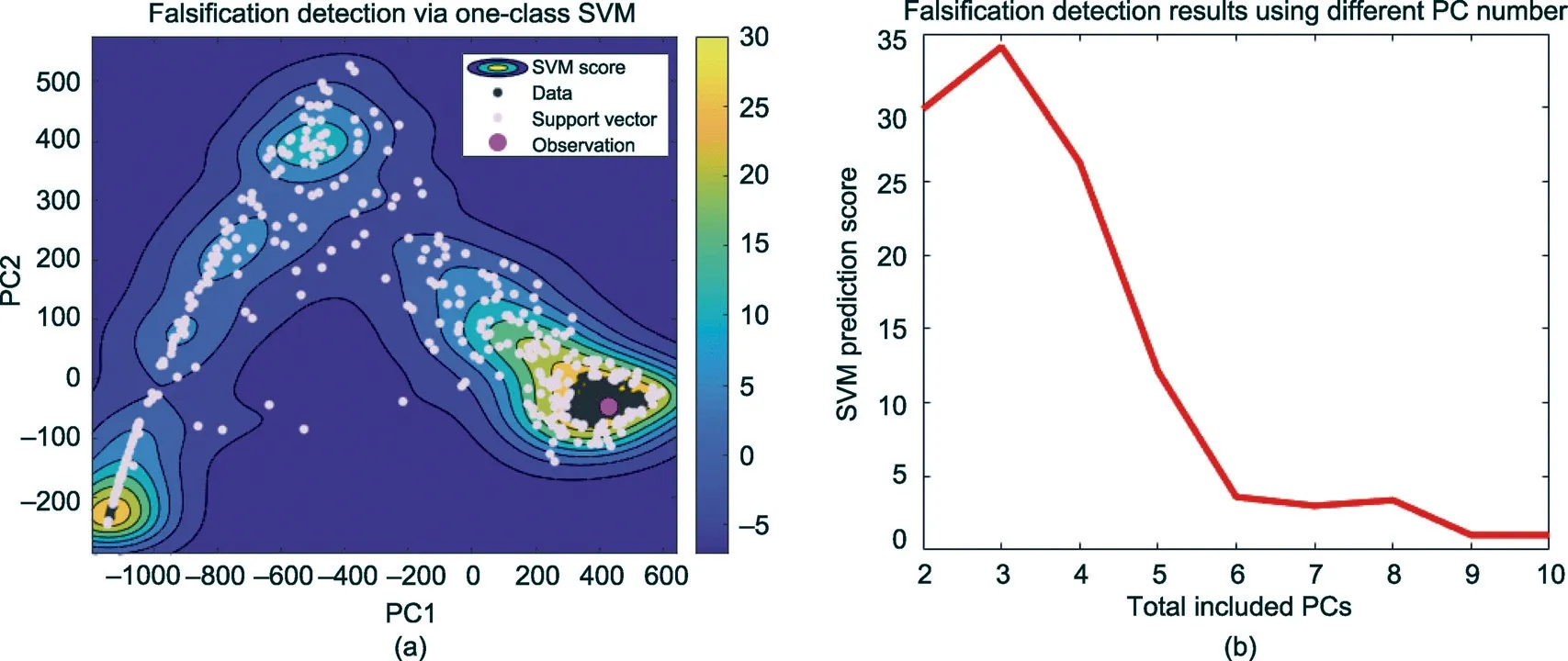
Fig.8. Outlier detection using a one-class SVM.(a)SVM result using PC1 and PC2;(b)prediction score of the observation using the SVM model,considering high-dimensional PCs.
4.5. Surrogate model training
Bayesian theorem allows us to reduce the uncertainty by calculating the posterior distribution. In this study, we employ ABC to calculate the posterior distribution, which needs sufficient prior realizations.Thus,a surrogate model is required to build a statistical model between the parameters and the simulation result.Here,we employ two tree-based regression techniques—random forest and gradient boosting—to build the relationship between the parameters and the distance of the simulation curves to the observation.
We use all the uncertain parameters as inputs of the regression model.The target output(label)is the mismatch of the simulations to the observation;hence,our output is a scaler(a distance).All the data curves are scaled between zero and one before being aggregated to capture the features from different wells and different data types.
We use 75% of the samples as the training dataset and 25% as the testing set. Fig. 9 shows that the regression performance of the random forest model and that of the gradient boosting model do not have a significant difference, with correlation coefficients of 0.83(Fig. 9(a))and 0.85(Fig. 9(b)),respectively. The correlation coefficients of the testing dataset on the random forest and gradient boosting models are 0.72(Fig.9(a))and 0.77(Fig.9(b)),respectively. The gradient boosting regression model seems to have better performance on both the training and testing datasets.However,the random forest model has better performance on the samples with a smaller distance value, which is more important because those samples are closer to the observation.Fig.9(c)compares the ranking correction between the random forest model and the gradient boosting model.It can be seen that the random forest model has a better performance when considering the samples that are close to the observation.Thus,we select the random forest model as the surrogate model.
4.6. Posterior global parameter distribution and data
Posterior distributions of the parameter are calculated via the ABC method. First, we generate 50 000 realizations of the prior parameters. The predicted distance is then calculated via the random forest model. In the ABC procedure, we use the value of 1.1 as the criterion to select the posterior samples (Fig. S14 in Appendix A).Fig.10 compare the posterior distribution of some sensitive parameters (e.g., fracture aperture, oil density, and fault modification of the area of wells P1 and P2)to their prior distribution.There are significant reductions in the uncertainty for the sensitive parameters.
Finally, to validate whether the uncertainty reduction is efficient,we use the updated parameters to build geological and simulation models again, and then run an actual flow simulation.Fig.11 shows the simulation curves using the updated parameters.The results demonstrate that the whole workflow is valid,because the posterior curves are closer to the observation curves.To further improve the match, it is possible to reject the simulated realizations that are deemed too far from the production history.Computational complexity should be taken into account in matching the history.In this study,the average time for each modeling and simulation realization is about 30 min. Because we only use Monte Carlo simulation and not iterative matching, parallel computing can be used to speed up the generation of the prior and posterior models.

Fig.9. Surrogate model performance.(a)Random forest;(b)gradient boosting;(c)rank correlation of random forest and boosting models.Blue dots in(a)and(b)represent the prediction performance on the training dataset, while orange dots represent the prediction performance on the testing dataset.
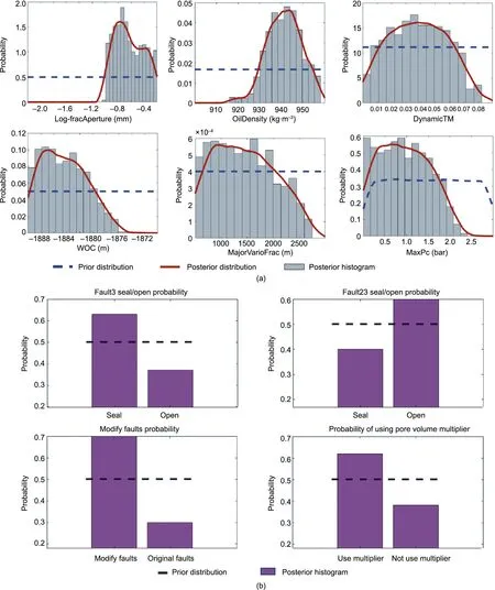
Fig. 10. Prior and posterior distributions of (a) the sensitive continuous parameters and (b) categorical sensitive parameters.
5. Discussion and conclusions
Falsification of the prior has been of concern in several field case studies[24,42,49].In field applications,especially for cases we have little knowledge of,a non-falsified prior must be stated.In this study,we considered many uncertainties in the initial prior.Even then,it turned out that the prior was falsified. Many papers on history matching do not mention the falsification step.Usually,ad hoc modification is done but not published; only the application of a technique is studied, and its success is emphasized. However, this is usually not the most essential problem engineers face in real cases.
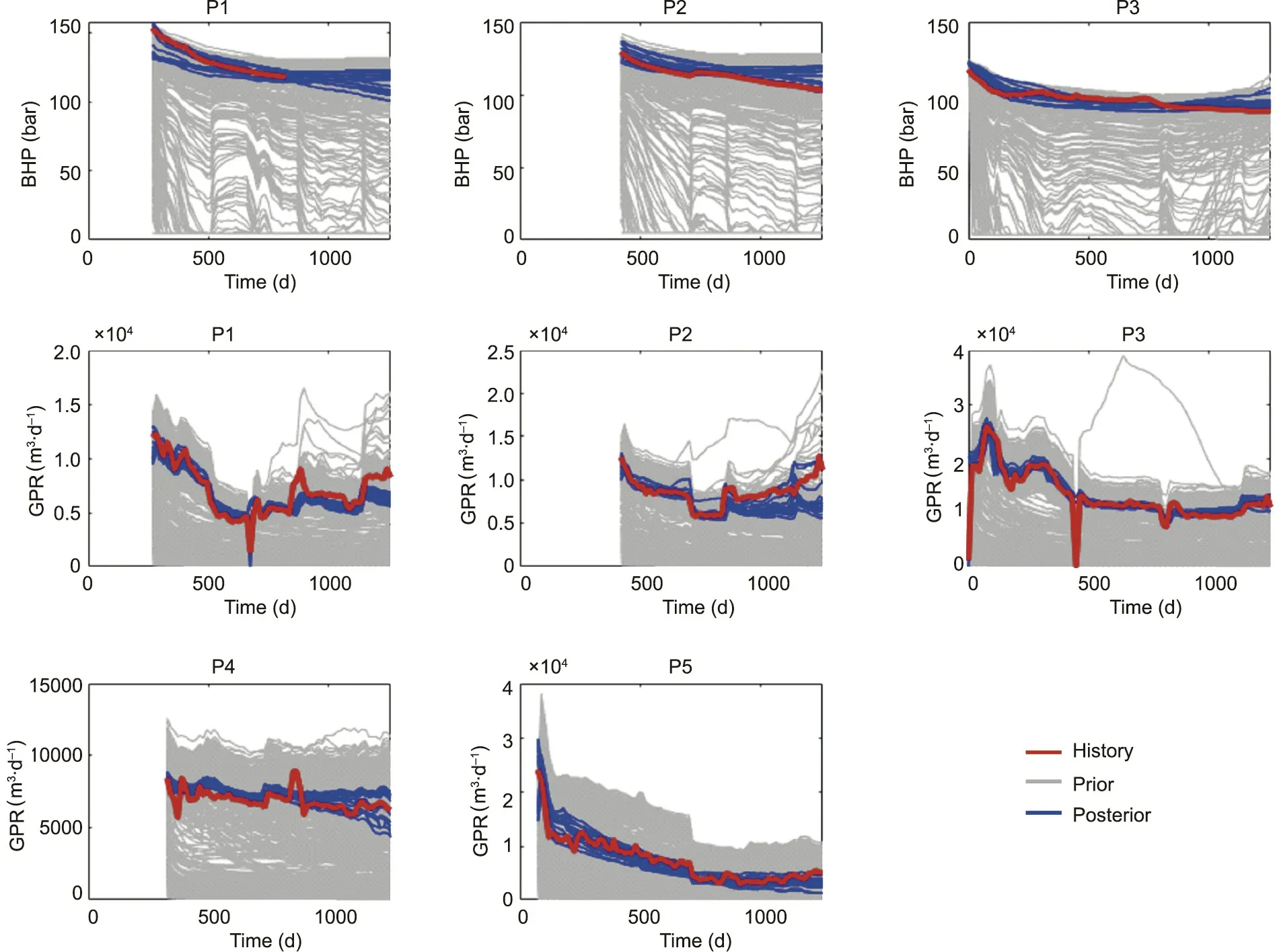
Fig. 11. Simulation data curves using posterior parameters.
In the de-falsification processes, it is easy to identify the problem of too-narrow distributions of the current uncertain parameters by using a sensitivity analysis and dimension reduction, such as the fracture aperture problem in Hypothesis 1 (Section 4). The more challenging part is to discover the important uncertainties that are ignored in the prior definition,which requires a great deal of domain knowledge and experience. For example, in this study,we consider the fault positions and connectivity to be certain in the initial prior.Without domain knowledge of seismic interpretation,a data scientist or a reservoir engineer would find this identification challenging. The alternative way is to have deep discussions with experts from different domains to determine the uncertainties in each domain, such as seismic interpretation,well logging interpretation, and production management.
Considering the computational complexity of the modeling and simulation,we generated 1000 realizations and then used a surrogate model. A statistical surrogate model will always decrease the uncertainty reduction performance. We used tree-based surrogate models because some input parameters are categorical. However,the tree-based regression model sacrifices some regression accuracy,as it uses a piecewise average in each node.A surrogate model will not be required if the geological model and forwarding simulation time is tolerable to run tens of thousands to millions of realizations.
In conclusion, we proposed a systematic approach to diagnose the falsification problem of the prior in the uncertainty quantification of a real fractured reservoir case.The proposed approach integrates GSA, dimension reduction, and Monte Carlo sampling. We demonstrated that the method is efficient in identifying the toosmall uncertainty of a stated prior and the deficiency of model complexity. More importantly, this method can diagnose the conflict that remains in the field data, such as the fault interpretation and production history in this study, as such conflict often occurs in field geological studies where the data of different aspects are measured.
Acknowledgment
We thank the China Scholarship Council, China University of Geosciences (Wuhan), Tracy Energy Technologies Inc., and Stanford Center for Earth Resources Forecasting for their support for this research. The authors would like to express special thanks to Markus Zechner, Zhen Yin, and Yizheng Wang for technical discussions and support.
Compliance with ethics guidelines
Junling Fang, Bin Gong, and Jef Caers declare that they have no conflict of interest or financial conflicts to disclose.
Appendix A. Supplementary data
Supplementary data to this article can be found online at https://doi.org/10.1016/j.eng.2022.04.015.
- Engineering的其它文章
- Editorial for the Special Issue on Unconventional and Intelligent Oil and Gas Engineering
- On-Chip LiDAR Technology Advances for Cars, Cell Phones
- Genetic Engineering Aims to Take a Bite Out of Insect Pests
- Two New Mega Dams Begin Operating as Hydropower Industry Booms
- Management Mode and Application of Geoscience-Engineering Integration
- Intelligent Petroleum Engineering

