Maximal Operator of (C,α)-Means of Walsh-Fourier Series on Hardy Spaces with Variable Exponents

ZHANG Xueying(张学英) ZHANG Chuanzhou(张传洲)

( 1.College of Science, Wuhan University of Science and Technology, Wuhan 430065, China;2.Hubei Province Key Laboratory of Systems Science in Metallurgical Process,Wuhan University of Science and Technology, Wuhan 430081, China)

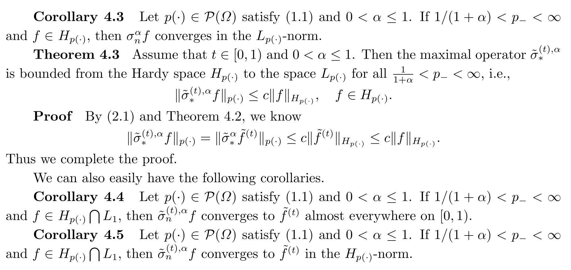
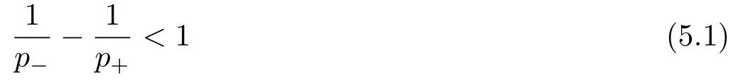
Abstract: In this paper, we consider the maximal operator of (C,α)-means of Walsh-Fourier series on Hardy spaces with variable exponents.For 0 ＜α ≤1,0 ≤t ＜1 the boundedness of the maximal operator and conjugate maximal operator on Hp(·)and Hp(·),q are proved whenever p- ＞1/(1+α) and the conditionholds.As a consequence, we obtain theorems about almost everywhere and norm convergence of thef and f.

Key words: (C,α)-kernel; Variable exponent; Maximal operator; Conjugate maximal operator

1.Introduction

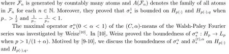
Variable Lebesgue spaces are a generalization of the classicalLpspaces, replacing the constant exponentpwith an exponent functionp(·).These spaces introduced by Orlicz[8]in 1931 have been the subject of more intensive study since the early 1990s, because of their intrinsic interest.Although the theory of variable Hardy spaces on Rnhas rapidly been developed in recent years, the variable exponent framework has not yet been applied to the martingale setting.The first main difficulty is to find a suitable replacement for the log-Hlder continuity condition when the variable exponentp(·) is defined on a probability space.In [9],the authors introduced a condition without metric characterization ofp(·) to replace the log-Hlder continuity condition mentioned above.They supposed that there exists a constantKp(·)≥1 depending only onp(·) such that

2.Definitions and Notations

A measurable functionp(·):[0,1)→(0,∞) is called a variable exponent.For a measurable setA ⊂[0,1), we denote

and for convenience

p-:=p-([0,1)), p+:=p+([0,1)).

Denote byP([0,1)) the collection of all variable exponentsp(·) such that 0＜p- ≤p+＜∞.

Definition 2.1The variable Lebesgue spaceLp(·)=Lp(·)([0,1)) is the collection of all measurable functionsfdefined on [0,1) such that for someλ ＞0,

with

Now let (Ω,F,P) be a complete probability space, whereΩ= [0,1) .By a dyadic interval, we mean one of the form [k2-n,(k+1)2-n) for somek,n ∈N,0≤k ＜2n.Givenn ∈N andx ∈[0,1), letIn(x) denote the dyadic interval of length 2-nwhich containsx.Theσ-algebras generated by the dyadic intervals{In(x) :x ∈[0,1)}will be denoted byFn(n ∈N).We know such (Fn)n≥0is regular and the elements of [0,1) are sequences of the form (x0,x1,··· ,xk,···),wherexk ∈{0,1}for everyk ∈N.The expectation and the conditional expectation operators relative toFnare denoted byEandEn, respectively.

A sequence of measurable functionsf=(fn)n≥0∈L1is called a martingale with respect to (Fn)n≥0ifEn(fn+1)=fnfor everyn ≥0.For a martingalef=(fn)n≥0, letf-1:=0 and

dnf=fn-fn-1,n ≥0.

If in additionfn ∈Lp(·), thenfis called aLp(·)-martingale with respect to (Fn)n≥0.In this case, we set

For a martingale relative to (Ω,F,P;(Fn)n≥0), we define the maximal function, the square function and the conditional square function off, respectively, as follows:

The variable martingale Hardy spaces associated with variable Lebesgue spacesLp(·)are defined as follows:

Next we introduce the definition of Lorentz spacesLp(·),q(Ω) with variable exponentsp(·)∈P(Ω) and 0＜q ≤∞is a constant.For more information about general casesLp(·),q(Ω), we refer the reader to [11].

Definition 2.2Given anF-measurable functionfon (Ω,F,P), define

LetA ∈F.A simple calculation above shows that

‖χA‖p(·),q ≈‖χA‖p(·).

Similarly, the variable martingale Lorentz-Hardy spaces associated with variable Lorentz spacesLp(·),qare defined as follows:

The product system generated by the Rademacher functions is the Walsh system:

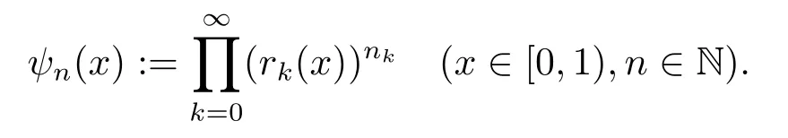
We remark that{ψn:n ∈N}is a complete orthogonal system on [0,1).

Recall that the Walsh-Dirichlet kernels

Dn:=ψn

satisfy

Iff ∈L1[0,1) then the number:=E(fψn)(n ∈N) is said to be thenth Walsh-Fourier coefficients off.We can extend this definition to martingales in the usual way (see[13]).

Denote bysnfthenth partial sum of the Walsh-Fourier series of a martingalef,namely,

It is easy to see thats2nf=fn.

Let

Then thenth partial sum of the conjugate transforms is given by

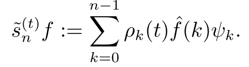
If 2N ≤n ＜2N+1, then we get immediately that

Forα-1,-2,··· ,let

It is known that

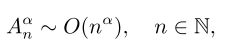
(see [14]).The (C,α) means of a martingalefare defined by

It is simple to show that

where the (C,α) kernel is defined by

Note that⊕denotes the dyadic addition (for the definition, see [15]).

The conjugate (C,α) means of a martingalefare introduced by

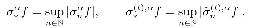
The maximal operator and the conjugate maximal operator are defined by

We also define the operator

whereIk,n=[k2-n,(k+1)2-n)=Ik,n ⊕[2-j-1,2-j-1⊕2-i), 0≤k ＜n,k ∈N.

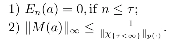
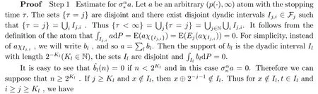
Definition 2.3Letp(·)∈P(Ω).A measurable functionais called a (p(·),∞)-atom if there exists a stopping timeτsuch that

3.Auxiliary Propositions

We shall need the following lemmas.

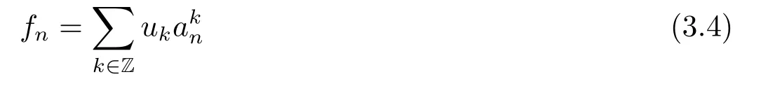
Lemma 3.1[9]Letp(·)∈P(Ω) satisfy (1.1) and 1＜p- ≤p+＜∞.For a fixed 0＜t ＜min{1,p-}andf= (fn)n≥0∈Hp(·), there exists a sequence of (p(·),∞)-atoms(ak)k∈Zassociated with stopping times (τk)k∈Zand a sequence of positive numbersuk=3·2k‖χ{τk＜∞}‖p(·)for eachksuch that

and

where the infimum is taken over all the decompositions off.

Lemma 3.2[9]Letp(·)∈P(Ω) satisfy (1.1) and 0＜t ＜min{p-,1}.Suppose that sublinear operatorT:L∞→L∞is bounded and

whereτkis the stopping time associated with (p(·),∞)-atomak.Then we have

‖Tf‖p(·)≤c‖f‖Hp(·), f ∈Hp(·).

Lemma 3.3[9]Letp(·)∈P(Ω) satisfy (1.1) and 1＜p- ≤p+＜∞and 0＜s,t ＜∞.Ifthen

Lemma 3.4[10]For 0＜α ≤1, we have

Lemma 3.5[9]Letp(·)∈P(Ω) satisfy (1.1) and 1＜p- ≤p+＜∞.Iff= (fn)n≥0∈Hp(·),q, there exists a sequence of (p(·),∞)-atoms (ak)k∈Zassociated with stopping times(τk)k∈Zand a sequence of positive numbersuk=3·2k‖χτk＜∞}‖p(·)for eachksuch that

and

where the infimum is taken over all the decompositions off.

Lemma 3.6[9]Letp(·)∈P(Ω) satisfy (1.1), 0＜q ＜∞.Suppose that sublinear operatorT*:L∞→L∞is bounded and

for some 0＜β ＜1.Then

‖T*f‖p(·),q ≤c‖f‖p(·),q, f ∈Hp(·),q.

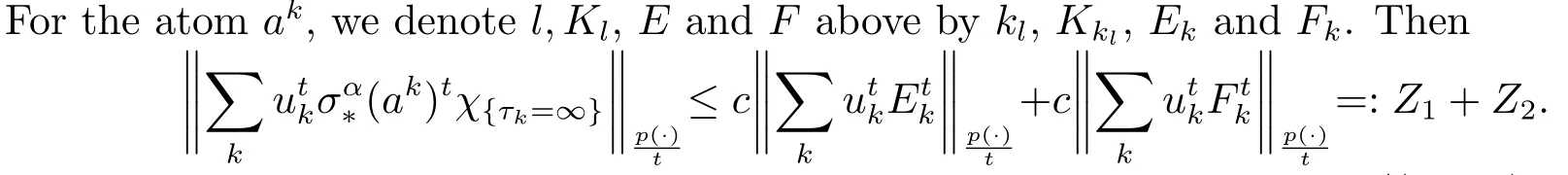
4.Maximal Operator on Variable Hardy Spaces

Theorem 4.1Letp(·)∈P(Ω) satisfy (1.1) and 1/(1+α)＜t ＜min{p-,1}.If

then

whereτkis the stopping time associated with (p(·),∞)-atomak.

Sincen ≥2Kl, we can chooseNsuch that 2N ＞n ≥2N-1.We haveN -1≥Kl.Hence by(2.8),

ifi ≥Kl, therefore,

By the following fact that

we have

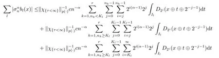
Consequently, forx ∈{τ=∞},

Step 2 Estimate forZ1.In this estimate, we have to usep- ＞t ＞1/(1+α).

Take max{1,p+} ＜r ＜∞large enough such that (1+α)t ＞r/(r-t).Then by Hder’s inequality andμk=3·2k‖χ{τk＜∞}‖p(·), we have

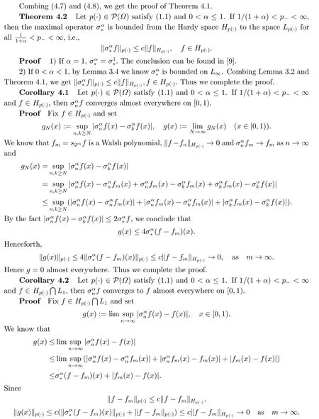
Henceg=0 almost everywhere.Thus we complete the proof.

For the norm convergence, we can prove the following consequences similarly, and we omit the proof.

5.Maximal Operator on Variable Hardy-Lorentz Spaces

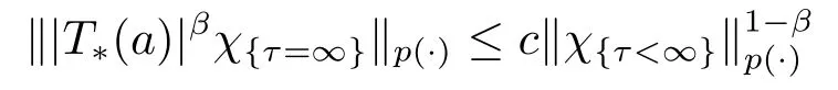
Theorem 5.1Let 0＜α ＜1,p(·)∈P(Ω)satisfy(1.1)and 1/(1+α)＜p- ＜p+＜∞.If

then

for some 0＜β ＜1 and for all (p(·),∞)-atomsa, whereτis the stopping time associated witha.

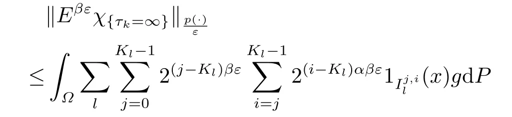
ProofFor 1/(1+α)＜ε ＜min{p-,1}, we can choose 0＜β ＜1 such thatβε ＞1/(1+α).Since

We choose max{1,βp+} ＜r ＜∞large enough such that (1+α)βε ＞r/(r-βε).Then by Hlder’s inequality we have

whenever

The estimate for

can also be found in [9].Combing (5.6) and (5.7), we complete the proof.

Theorem 5.2Let 0＜α ≤1,p(·)∈P(Ω)satisfy(1.1)and 1/(1+α)＜p- ＜p+＜∞.If

Similarly, for the conjugate operator, we also have

Theorem 5.3Lett ∈[0,1), 0＜α ≤1,p(·)∈P(Ω) satisfy (1.1) and 1/(1+α)＜p- ＜p+＜∞.If