Implementation of absorbing boundary conditions in dynamic simulation of the material point method*

Zhi-gang SHAN, Zhe-xian LIAO, You-kou DONG†‡, Dong WANG, Lan CUI

Implementation of absorbing boundary conditions in dynamic simulation of the material point method*

Zhi-gang SHAN1,2, Zhe-xian LIAO3,4, You-kou DONG†‡3,4, Dong WANG5, Lan CUI6

College of Marine Science and Technology, China University of Geosciences, Wuhan 430074, China Hubei Key Laboratory of Marine Geological Resources, China University of Geosciences, Wuhan 430074, China College of Environmental Science and Engineering, Ocean University of China, Qingdao 266100, China State Key Laboratory of Geomechanics and Geotechnical Engineering, Institute of Rock and Soil Mechanics, Chinese Academy of Sciences, Wuhan 430071, China †E-mail: dongyk@cug.edu.cn

Outgoing waves arising from high-velocity impacts between soil and structure can be reflected by the conventional truncated boundaries. Absorbing boundary conditions (ABCs), to attenuate the energy of the outward waves, are necessary to ensure the proper representation of the kinematic field and the accurate quantification of impact forces. In this paper, damping layer and dashpot ABCs are implemented in the material point method (MPM) with slight adjustments. Benchmark scenarios of different dynamic problems are modelled with the ABCs configured. Feasibility of the ABCs is assessed through the velocity fluctuations at specific observation points and the impact force fluctuations on the structures. The impact forces predicted by the MPM with ABCs are verified by comparison with those estimated using a computational fluid dynamics approach.

Material point method (MPM); Absorbing boundary condition (ABC); Submarine landslide; Impact

1 Introduction

The material point method (MPM) was developed to tackle the mesh distortion in large deformation problems, by combination of a fixed Eulerian mesh and clouds of Lagrangian particles flowing through the mesh (Sulsky et al., 1995; Soga et al., 2016). In calculations, the history state of the particles is derived from the temporary information on the surrounding nodes, while the nodes are fixed in space. Therefore, the MPM can avoid the mesh distortion and the necessary remeshing of the conventional finite element methods (Hu and Randolph, 1998). In comparison with other large deformation methods, such as coupled Eulerian-Lagrangian (Zheng et al., 2015), smooth particle hydrodynamics (Bui et al., 2008), and particle finite-element method (Zhang et al., 2013), the MPM has a higher demand for computational resource since it often utilizes very fine meshes. Excessive compression or tension in the kinematic field tends to entangle the particles from the initial uniform configuration, causing artificial voids or aggregations that lead to loss of the continuity of the stress field and the singular deformation gradient of the particles (Dong, 2020). Recently, the MPM has been used to simulate high-velocity impact in geotechnical engineering, such as submarine landslides impacting subsea structures (Dong et al., 2017a, 2017b) and the dynamic process of pile driving (Hamad et al., 2015). However, truncated boundaries with the conventional inflow or roller conditions were employed in most of the existing MPM simulations of impacts, and thus a sufficient distance from the region of concern to the boundary is required to accommodate the propagation of elastic waves. The computational efforts caused may become unacceptable, even when the central processing unit (CPU) and graphics processing unit (GPU) parallel strategies boosting the computational efficiency are used (Huang et al., 2008; Dong et al., 2015; Dong and Grabe, 2018; Gao et al., 2018).

Various absorbing boundary conditions (ABCs), such as the periodic boundary condition (Longuet- Higgins and Cokelet, 1976), infinite element scheme (Astley et al., 2000), and Dirichlet-to-Neumann radiation condition (Oberai et al., 1998), have been proposed to absorb the energy of the outgoing elastic waves on the far-field boundary. The dashpot boundary condition, one of the most popular ABCs (Lysmer and Kuhlemeyer, 1969; Kouroussis et al., 2011), might be the only ABC that has been implemented in the MPM simulations due to its robustness (Shen and Chen, 2005; Jassim et al., 2013; Bisht and Salgado, 2018). However, the dashpot ABC was imposed on the boundary nodes in terms of viscous tractions with velocities mapped from the associated particles, which is computationally intensive and hard to parallelize (Dong et al., 2015). Creeping motion caused by low frequency waves was avoided by setting a spring on the boundary node (Kellezi, 2000). Although it has been proven to be suitable for free and fixed boundaries, the dashpot ABC is difficult to extend to specific scenarios, such as open channel flows with velocity inflow boundaries. Additionally, for waves approaching the boundary at angles oblique to normal, the dashpot ABC is less effective as many other ABCs (Bisht and Salgado, 2018).

The damping layer ABC, originally developed for time-domain explicit solving of electromagnetic signal processing (Berenger, 1994), is efficient in absorbing the waves at grazing incidence to the boundary. It was widely applied in spectral analysis of seismic waves (Komatitsch and Tromp, 2003) and fluid-structure interactions. An artificial dissipative term is utilized in the damping layer of finite thickness to attenuate the amplitude of the outgoing waves. The formulation is local in both space and time, which renders the damping layer ABC computationally inexpensive, easy to implement, and robust. The damping layer ABC is more flexible than the dashpot and similar ABCs, which can be imposed on most boundaries of viscoelastic materials (Altomare et al., 2017; Wang et al., 2019). Therefore, the damping layer ABC has been incorporated into the finite element method (Yao et al., 2018), finite volume method (Sankaran et al., 2006), and smooth particle hydrodynamics (Altomare et al., 2017). However, computational instability may be induced by the residual stress waves through the damping layers in anisotropic media (Bécache et al., 2003; Meza-Fajardo and Papageorgiou, 2008), which need to be enhanced with special treatment (Gao and Huang, 2018). Additionally, the dissipation ratio of the damping layer has to be enforced in a gradual manner from the source domain to the boundary to avoid spurious wave reflections due to the inhomogeneity introduced (Festa et al., 2005; Komatitsch and Martin, 2007). Therefore, feasible configuration of the damping layer needs to be determined and then its performance in the MPM simulations should be investigated.

In this paper, a combination of the dashpot and damping layer ABCs is incorporated into the MPM. The feasibility of each ABC is investigated in terms of different dynamic scenarios. Only elastic waves are considered; plastic ones are not the concern of this work. The outgoing impacting wave is characterized as a compressional wave rather than a shear wave since the transportation of the former is much faster. The absorbing effect of the ABCs is quantified by the attenuation of the velocity fluctuations at specific locations and that of the impact force fluctuations in structure-soil interactions.

The remainder of this paper is organized as follows. In Section 2, detailed operations to implement the ABCs are described. Section 3 assesses the absorbing effect and the feasibility of different ABC configurations. Section 4 lists the concluding remarks and principal findings.

2 Implementation

An in-house MPM program has been developed, which features a novel contact algorithm ‘Geo-contact’ (Ma et al., 2014), a GPU parallel computing strategy (Dong et al., 2015; Dong and Grabe, 2018), and reseeding of over-sparse or dense particles (Dong, 2020). The explicit updated Lagrangian calculation in each incremental step is based on the generalized interpolation material point (GIMP) method presented by Bardenhagen and Kober (2004). This program was used to simulate the impact of submarine landslides on pipelines and foundations partially buried in the seabed (Dong et al., 2017a; Dong, 2020). The dashpot and damping layer ABCs (Fig. 1), with potential to be implemented in the MPM, are developed here.

The dashpot ABC can be used for either free or fixed boundaries, but not for velocity inflow boundaries. The viscous traction required to absorb the wave energy is (Shen and Chen, 2005)

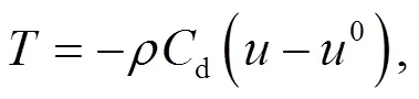
whereis the density;0andare the steady and transient velocities of the soil along the wave direction, respectively;dis the velocity of the wave, which for elastic material is defined as

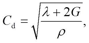
withas shear modulus andas Lamé’s parameter.

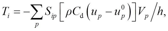
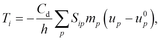
In the MPM, the traction in Eq. (1) was previously imposed on layers of boundary nodes with the velocities mapped from the associated particles (Fig. 1) (Shen and Chen, 2005; Bisht and Salgado, 2018)

To implement the damping layer ABC, a damping ratioβwas assigned at each nodein a lengthfrom the boundary of the material; the transient nodal velocityualong the wave direction was then explicitly modified as

The damping ratio needs to be sufficiently small at the starting surfaces of the damping layer to avoid potential reflections. Its value at nodeagainst the outgoing waves increased linearly with the distance to the boundary:

whereis a fitting coefficient, anddis the distance of nodeto the boundary. The parametersandin Eq. (7) need to be optimized through trial calculations in specific scenarios to allow for a minimum wave reflection. The minimum requirement of the damping layer lengthis often proportional to the wave length (Rajagopal et al., 2012). Differently from Eq. (7), an exponential growth of the damping ratio with the distance to the boundary was derived by Chern (2019). In each incremental step of the MPM calculation, the particle velocities are firstly mapped to the surrounding nodes (refer to Dong (2020) for detailed description of the MPM algorithm); then, the dashpot or damping layer ABC can be implemented by adjusting the nodal velocities using Eqs. (5) and (6); after calculating the governing equations on the nodes, the new velocity field is mapped from the nodes to particles. Given that a quadratic shape function is used, an additional layer of ghost cells out of the material boundary is configured to implement the boundary conditions (Fig. 1). Parallelization of Eqs. (5) and (6) becomes straightforward by splitting the whole workload over the nodes with the computation in the threads independent to each other.

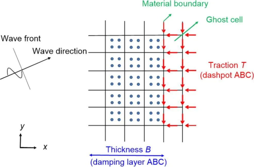
Fig. 1 Implementation of ABCs

3 Benchmark

3.1 One-dimensional compression

A block of elastic material with 50 m in width and height (Fig. 2) was compressed vertically under a velocity pulse=sin(2π) (0≤≤0.5 s) on its top surface, whereis the time. The density of the material was 650 kg/m3, Young’s modulus was 150 kPa, and Poison’s ratio was 0.3. The lateral boundaries were considered as symmetric, while the top as free. The bottom boundary was initially configured with rollers, which were then replaced with the dashpot and damping layer ABCs. The element size in the MPM model was 1 m with four particles seeded in each element prior to the calculation.

The stress wave induced by the pulse propagates from the top surface to the bottom (Fig. 3). The elapse time of the wave from point(at height of 50 m) to point(at height of 5 m) is 0.7 s (Fig. 4), which hints a propagation speed of 64 m/s. This is consistent with the material properties stated above, which give a compressional wave speed of 63 m/s using Eq. (2). Given the reflective boundary condition (BC) of rollers imposed at the bottom of the material, the compressional wave is retained in the material since it is purely elastic. With the dashpot and damping layer (such as=0.01,=10 m) ABCs configured, the stress wave was absorbed within two periods of transportation. The magnitudes of residual stress waves at=3 s are less than 15% of their original values at pointsand. After 3 s, the residual wave can be ignored. Therefore, both the two ABCs are effective to attenuate the stress waves in elastic materials for the 1D compression problems. In comparison, the dashpot ABC slightly outperforms its damping layer cousin in terms of absorbing efficiency.

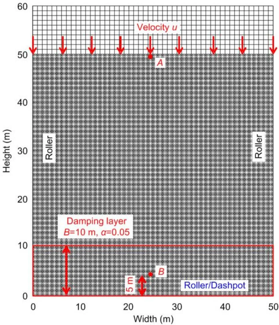
Fig. 2 Compression of material under velocity pulse

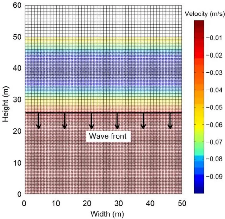
Fig. 3 Velocity contour in material at t=0.4 s

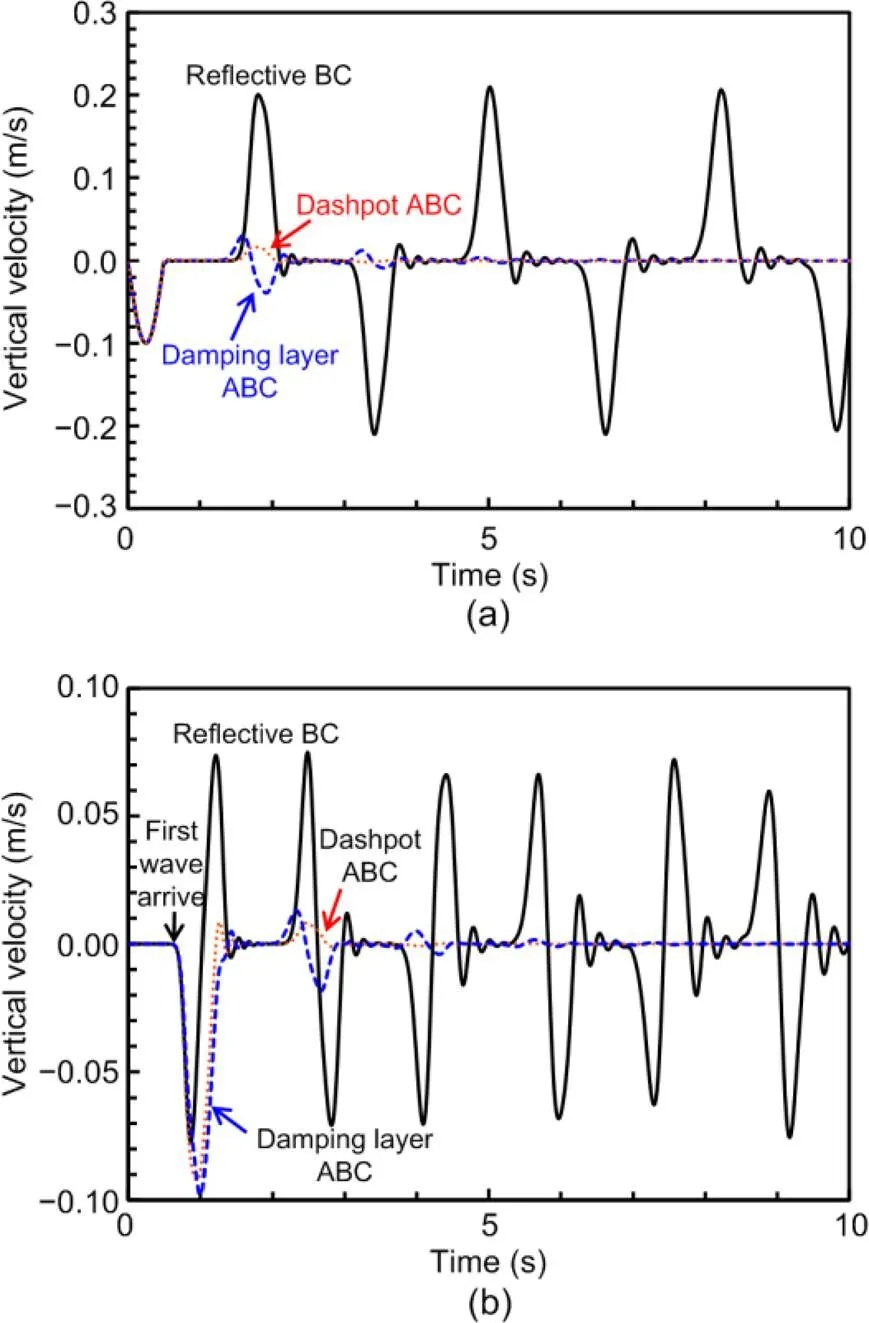
Fig. 4 History of velocity at observation points with different boundary conditions

(a) Point; (b) Point

3.2 Submarine landslide impacting mudmat

Simulation of submarine landslide impacting subsea mudmat was performed with a schematic of the initial conditions provided in Fig. 5a. A rectangular block of sliding mass with a lengthof 20 m and a height of 10 m was assumed on a smooth rigid base. The sliding mass was given a horizontal velocity=6 m/s. A velocity inflow boundary condition was enforced at the left end of the sliding mass, while the upper and right surfaces were free. A planar mudmat of finite length of 10 m, partially buried with an exposure height of=1 m, was placed immediately in front of the sliding mass. The element size was selected as/40. The mesh independency of the impact force on the element size has been studied in (Dong et al., 2017b). A 4×4 particle configuration was allocated for each element fully occupied by the sliding mass; therefore, there were 5.1 million slide particles configured.

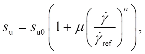
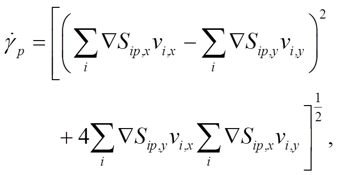
The rate-dependent undrained shear strength of the non-Newtonian sliding material is characterized by the Herschel-Bulkley (H-B) rheological model and implemented with the von Mises criterion by expanding the yield surface:

The density of the sliding mass was=1500 kg/m3. The gravity acceleration was=9.81 m/s2. Considering buoyancy, the effective unit weight of the material was (−w), wherewis the density of water. Poisson’s ratio of the sliding mass was taken as 0.49, and Young’s modulus was 300u0. The time step Δwas determined through the Courant-Friedrichs-Lewy stability condition with the Courant number as 0.4.

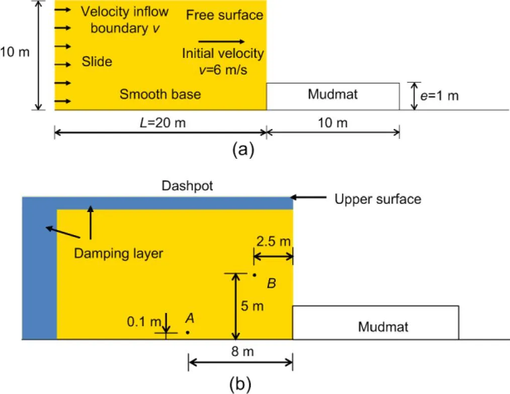
Fig. 5 Schematic for submarine landslide across mudmat (non-scaled)

(a) Initial conditions; (b) Setup of ABCs

The robustness of our MPM program without the ABC was verified by comparison with computational fluid dynamics (CFD) simulations, where the elastic wave propagation is avoided by an incompressible framework (Dong et al., 2017b). The impact pressures on the mudmat,, predicted by the CFD and MPM analyses without ABCs are normalized with the inertia of the sliding mass2, as shown in Fig. 6. The pressures in the CFD analyses at the very early stage are virtually infinite, while the impact pressure rises rapidly to a peak value before 0.01 s in the MPM analyses. Impact waves are generated by the sudden interaction between the sliding mass and the mudmat (Fig. 7a), and propagate towards the upper and left boundaries (Figs. 7b and 7c). The speed of the compressional waves can be estimated with Eq. (5) as 41.2 m/s. Therefore, the first waves reflected by the upper and left boundaries arrive at the sliding mass– mudmat interface at about 0.44 and 0.84 s with considering the sliding velocity of 6 m/s, which are consistent with the emergence of pressure fluctuations in Fig. 6. The pressures predicted by the MPM are close to the CFD predictions before 0.44 s. After that the MPM predictions present severe fluctuations due to the wave reflection.

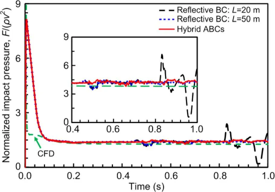
Fig. 6 Normalized impact pressures predicted by CFD and MPM simulations

Fig. 7 Contours of slide velocities

(a)=0.05 s; (b)=0.30 s; (c)=0.53 s

3.2.1 Effect of the left boundary

The wave reflections at the left boundary can be delayed if a longer length of the sliding mass is considered. With=50 m, the waves reflected by the left boundary are expected to arrive at the sliding mass–mudmat interface at about 2.1 s. The remaining pressure fluctuations at about 0.44 s with=50 m in Fig. 6 are mainly due to the wave reflection at the upper boundary. The MPM prediction with=50 m converges to the CFD counterpart, although larger length of the sliding mass means higher computational efforts.

Kinematic history of the upstream point(Fig. 5b) at the height of 0.1 m and the initial distance of 8 m to the mudmat is investigated (Fig. 8a). The outgoing compressional wave arrives at pointat about 0.18 s, causing fluctuations of the horizontal velocities with a maximum fluctuation magnitude of about 2 m/s. The wave elapses after 0.05 s, which corresponds to a wave length of 2 m. At the left end of the sliding mass with a velocity inflow boundary, the wave is reversed and returns to the sliding mass– mudmat interface given that the ABC is not imposed. As a result, an increase of the slide velocity emerges at pointat about 0.74 s. The velocity fluctuations at 0.5 s are induced by the wave reflections by the upper boundary; that aspect will be tackled later in this study.

To attenuate the outgoing waves at the left boundary of the sliding mass, the damping layer ABC is added with a total thickness=10 m and=0.005. The damping layer domain of nodes proceeds along with the sliding mass at a horizontal velocity of 6 m/s. Velocity of the particles in the damping layer was influenced by the velocity adjustment of the surrounding nodes by Eqs. (6) and (7). For the particles out of the damping layer, the velocity remained unchanged. The velocity fluctuations between 0.74 and 0.97 s for pointare significantly mitigated (Fig. 8a). The remaining fluctuations are caused by the residual wave through the damping layer. Further investigation was performed to study the effect of parametersandin Eq. (7) as shown in Fig. 9. With a smaller value of(e.g.=0.001) or a thinner damping layer (e.g.=5 m), the outgoing waves are under-damped; hence relatively high fluctuations of the sliding velocities are retained. With higher values of, such as 0.05, the outgoing waves are sufficiently damped, but transitional reflection of waves is caused by the sudden addition of the artificial damping, which arrives at pointearlier than the residual wave by about 0.5 s. Through trial calculations, the value ofis suggested to be 0.003–0.015 and≥7.5 m, which corresponds to 3.5 times the wave length. Since the dashpot ABC cannot be imposed on the velocity inflow boundary, its effect on the horizontal velocity at pointis not studied.

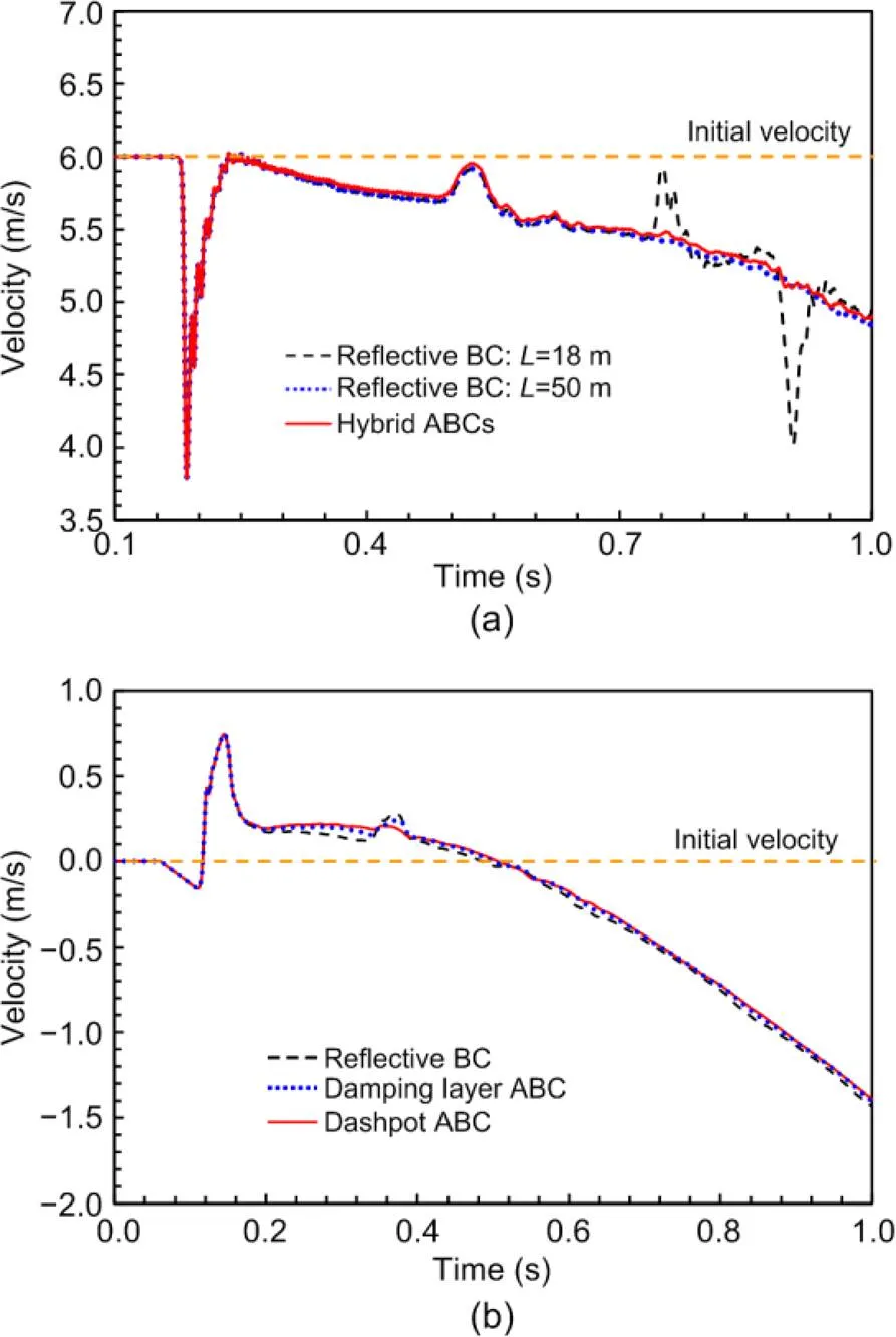
Fig. 8 Velocity profiles at observation points with different boundary conditions

(a) Horizontal velocity at pointwith left boundary conditions; (b) Vertical velocity at pointwith upper boundary conditions

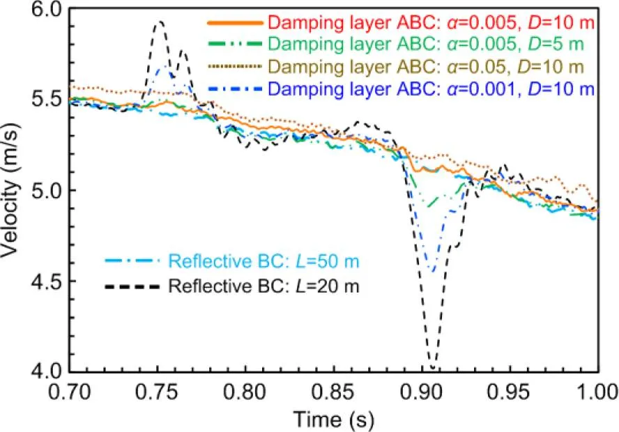
Fig. 9 Effect of configurations of damping layer ABC on horizontal velocity at point A

3.2.2 Effect of the upper boundary

The kinematic history of upstream pointat the height of 5 m and the initial distance of 2.5 m to the mudmat (Fig. 5b) is investigated (Fig. 8b). The outgoing compressional wave arrives at pointat about 0.11 s, causing fluctuations of the vertical velocities with a maximum fluctuation magnitude of about 0.5 m/s. The wave is reflected back to the slide mass with its shape retained. The reflected wave keeps propagating between the upper boundary and the base, which causes fluctuations of vertical velocities of pointat 0.34 and 0.52 s. The propagation of the wave along the height of the sliding mass also causes fluctuations of the horizontal pressures, which are the main reason for the fluctuations of the impact pressures on the mudmat at 0.44 s in Fig. 6.

To attenuate the wave reflection at the upper boundary, the damping layer ABC is added. The upper boundary at the front of the sliding mass is in a plastic zone (Fig. 7b), which means the elastic impact wave is transported along with the permanent plastic waves. Therefore, the damping layer needs to be sufficiently thin to avoid the complicated operations of wave-separation, such as=1 m and=0.005. However, with such a thin damping layer, the outgoing wave is under-damped as discussed in the previous section.

The dashpot ABC was added at the upper boundary of the sliding mass as shown in Fig. 5b. Since the upper surface of the sliding mass sinks in the sliding process due to the release of the static pressure, the upper layer of particles should be detected at each incremental step before implementing the dashpot ABC at the boundary nodes. The two layers of nodes beyond the upper layer of particles can be considered as the boundaries for implementing the dashpot ABC. With the dashpot ABC, the velocity fluctuations at pointdue to the residual wave are less than 10% of the original at 0.34 s (Fig. 8b). After 0.34 s, the velocities at pointare relatively stable, which implies that the residual wave is fully absorbed. With the dashpot ABC, the severe fluctuation of the impacting pressures at 0.44 s in Fig. 6 is also alleviated. Therefore, the dashpot ABC at the upper boundary, based on accurate derivations of wave equations, is more practical for free surfaces with a complex kinematic field than the damping layer ABC. In contrast, the damping layer ABC needs a sufficiently thick elastic zone in the kinematic field. A hybrid configuration of the ABCs can be imposed with a damping layer ABC on the left zone of the sliding mass and a dashpot ABC on the upper free boundary. With such a configuration, the impacting pressures predicted by the MPM are relatively stable and converge to the CFD prediction (Fig. 6). The velocity contour of the sliding mass with the ABCs is shown in Fig. 10, in which the impacting waves (Fig. 7c) are fully absorbed.

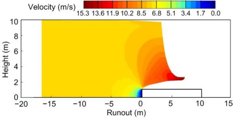
Fig. 10 Contour of velocities at 0.53 s with hybrid ABCs

3.3 Dynamic penetration of pipe

A smooth pipeline with a diameter=0.8 m was driven into clay from the surface. The submerged density of the soil was 650 kg/m3. The geostatic stresses induced by the self-weight of the soil were not considered. The clay was assumed as an elastic- perfectly plastic material with the von Mises yield criterion and with the size of the yield surface remaining unchanged. The undrained shear strength of the normally consolidated clay wasu=2.5 kPa. Poisson’s ratio of the soil was taken as 0.49, and Young’s modulus was 500u. The time step Δwas determined through the Courant-Friedrichs-Lewy stability condition with the Courant number of 0.4. In the MPM analysis, a half model was considered by taking advantage of the symmetry along the central line. Then the soil extensions in the horizontal and vertical directions were 3.125with the mesh size=0.0125(Fig. 11). Roller boundary conditions were initially assigned to the right and bottom boundaries of the soil, while the top boundary was free. A 4×4 particle configuration was allocated for each element fully occupied by the soil.

The pipe was driven into the soil at velocitiespipeof 0.1 (quasi-static) and 5 m/s (dynamic), respectively. The robustness of the MPM simulations would be verified by comparison of the obtained penetration resistancevon the pipe with CFD predictions (ANSYS, 2011). The dynamic meshing technique was used along with the void-of-fluid scheme as detailed in (Dong et al., 2017b). The penetration resistances predicted by the CFD and MPM analyses are normalized by the shear strength of the soil (Fig. 12), whereis the penetration depth of the pipe. The fluctuations, particularly in the CFD results, are mainly due to the errors in the recovery of state variables after re-meshing in each incremental step. In the MPM analyses, magnitudes of the stress waves are quite small for the quasi-static case; therefore, its prediction of the penetration resistance is quite smooth and agrees well with the CFD results. For the dynamic case, the fluctuations of the resistance at a shallow penetration (/<0.1) are mainly due to the establishment of the kinematic field under the initial impact. Then at/=0.172, the stress wave reflected by the bottom boundary returns to the pipe–soil interface, causing strong fluctuations in the resistance. This can be proven by the propagation velocity of the stress wave of 178 m/s as predicted by the properties of the soil. To remove the disturbance of the stress wave reflection before/=0.5, the width and height of the soil need to be larger than 7.12 m as calculated by (0.5×0.8/5)×178/2. Therefore, the minimum model dimensions are determined by the penetration period (/(pipe)) and the velocity of the stress wave (178 m/s). Then dashpot and damping layer ABCs were imposed on the bottom and lateral boundaries. In the damping layer additional materials of thickness=1 m were configured at the boundaries with the parameter=0.005, determined through trial calculations. The absorbing effect of the ABCs is generally satisfactory as the fluctuations of the resistance were attenuated significantly. The local fluctuations of the resistance at/>0.1 are controlled within 5%. The resistances predicted by the CFD are higher than the MPM counterpart for around 6%. This is attributed to the larger contact interface between the pipe and soil in the CFD model as a gap is not allowed between them in the void-of-fluid solver (Fig. 13). Therefore, the MPM is preferred to simulating the dynamic penetration of a structure. The velocity contours in the soil predicted by the CFD and MPM are shown in Fig. 13.

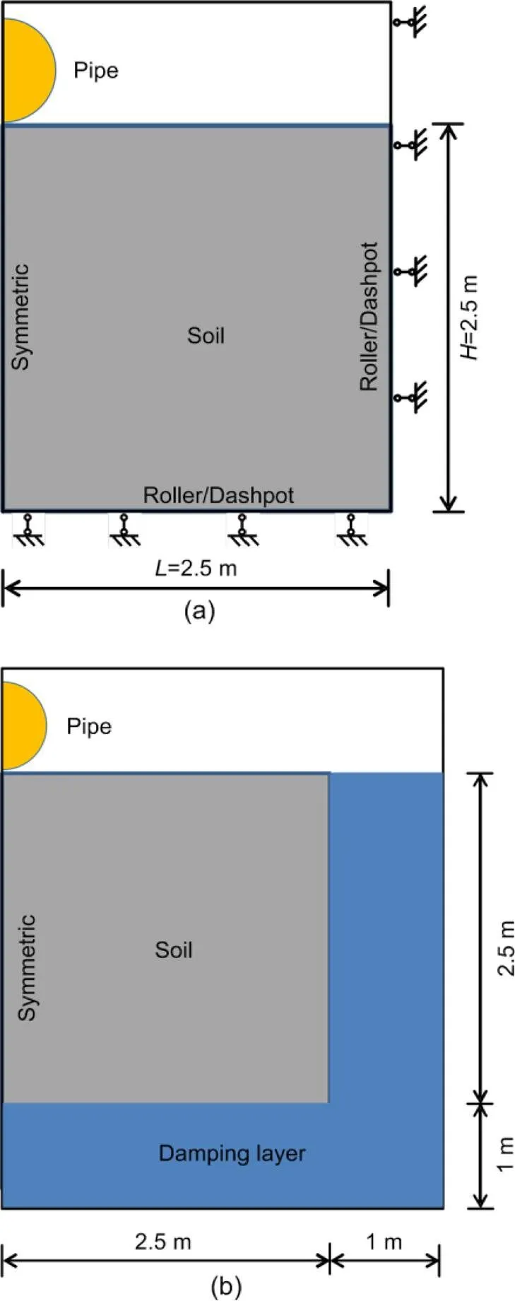
Fig. 11 Schematic for the pipe penetration into soil (non-scaled)

(a) Roller or dashpot boundary; (b) Damping layer boundary

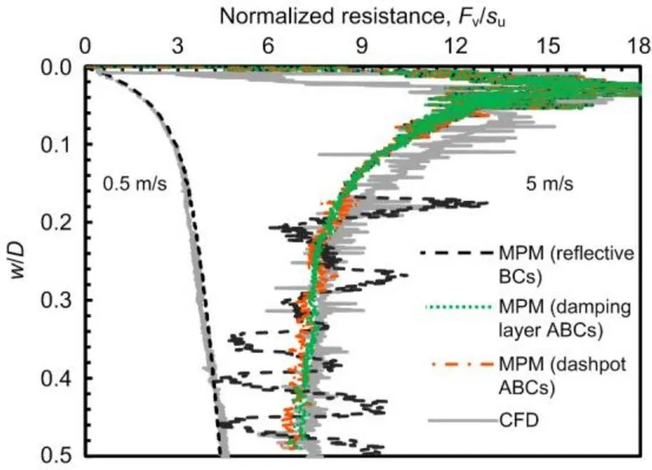
Fig. 12 Normalized penetration resistance predicted by CFD and MPM

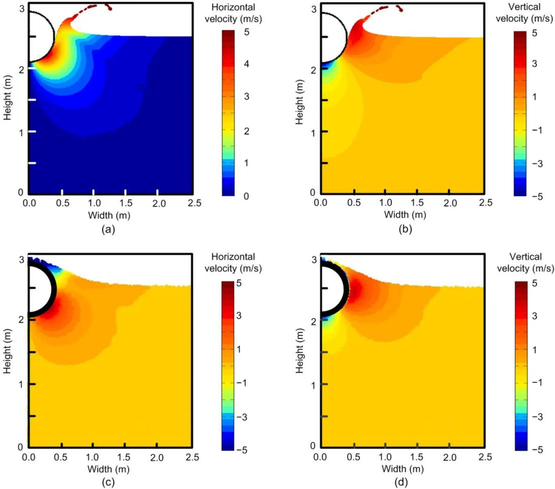
Fig. 13 Velocity contours predicted by MPM and CFD

(a) Horizontal velocity (MPM); (b) Vertical velocity (MPM); (c) Horizontal velocity (CFD); (d) Vertical velocity (CFD)

4 Conclusions

Dashpot and damping layer ABCs were implemented in the MPM to absorb the outgoing waves. The former was imposed on boundary nodes in terms of traction forces, while the latter utilized a damping layer of finite thickness inside the soil. Feasibility of the ABCs was assessed through benchmark problems of 1D compression, submarine landslides impacting mudmat, and dynamic penetration of a pipeline. Velocity fluctuations induced by elastic wave propagation and the impact force fluctuations on the structures were investigated at specific observation points. The dashpot ABC, based on accurate derivations of wave equations, is more feasible for free surfaces with a complex kinematic field than the damping layer ABC. In contrast, the damping layer ABC requires a sufficiently thick elastic zone in the kinematic field, and the damping ratio increased linearly with the distance to the boundary at a coefficient between 0.003 and 0.015. In specific scenarios, the two ABCs can be utilized together to adapt to different boundary settings. Finally, the impact forces predicted by the MPM with the ABCs were verified by comparison with those estimated using a CFD approach.

Contributors

You-kou DONG and Zhi-gang SHAN: conceptualization, methodology, validation, investigation, writing–original draft; Zhe-xian LIAO: data curation, formal analysis; Lan CUI: visualization, project administration; You-kou DONG and Dong WANG: writing–review & editing.

Conflict of interest

Zhi-gang SHAN, Zhe-xian LIAO, You-kou DONG, Dong WANG, and Lan CUI declare that they have no conflict of interest.

Altomare C, Domínguez JM, Crespo AJC, et al., 2017. Long- crested wave generation and absorption for SPH-based DualSPHysics model., 127:37-54. https://doi.org/10.1016/j.coastaleng.2017.06.004

ANSYS, 2011. ANSYS FLUENT Theory Guide, Release 14.0. ANSYS, Inc., Canonsburg, USA.

Astley RJ, Gerdes K, Givoli D, et al., 2000. Finite elements for wave propagation–special issue of the Journal of Computational Acoustics., 8(1):257.

Bardenhagen SG, Kober EM, 2004. The generalized interpolation material point method., 5(6):477-495.

Bécache E, Fauqueux S, Joly P, 2003. Stability of perfectly matched layers, group velocities and anisotropic waves., 188(2):399-433. https://doi.org/10.1016/S0021-9991(03)00184-0

Berenger JP, 1994. A perfectly matched layer for the absorption of electromagnetic waves., 114(2):185-200. https://doi.org/10.1006/jcph.1994.1159

Bisht V, Salgado R, 2018. Local transmitting boundaries for the generalized interpolation material point method., 114(11):1228-1244. https://doi.org/10.1002/nme.5780

Boukpeti N, White DJ, Randolph MF, et al., 2012. Strength of fine-grained soils at the solid-fluid transition., 62(3):213-226. https://doi.org/10.1680/geot.9.P.069

Bui HH, Fukagawa R, Sako K, et al., 2008. Lagrangian meshfree particles method (SPH) for large deformation and failure flows of geomaterial using elastic-plastic soil constitutive model., 32(12):1537- 1570. https://doi.org/10.1002/nag.688

Chern A, 2019. A reflectionless discrete perfectly matched layer., 381:91-109. https://doi.org/10.1016/j.jcp.2018.12.026

Dong Y, 2020. Reseeding of particles in the material point method for soil–structure interactions., 126:103716. https://doi.org/10.1016/j.compgeo.2020.103716

Dong YK, Grabe J, 2018. Large scale parallelisation of the material point method with multiple GPUs., 101:149-158. https://doi.org/10.1016/j.compgeo.2018.04.001

Dong YK, Wang D, Randolph MF, 2015. A GPU parallel computing strategy for the material point method., 66:31-38. https://doi.org/10.1016/j.compgeo.2015.01.009

旗帜鲜明讲政治、讲立场这是当代马克思主义理论的根本要求。红色文化促进了文化自信、道路自信、制度自信、理论自信,“筑牢信仰之基、补足精神之钙、把稳思想之舵，把共产党人的精神支柱和政治灵魂立起来”[6]。红色文化使英雄丰满，使故事感人，使情节真实，使理论阐述科学，能把人们带入历史叙事中去认知和切身感受，从而引发人民群众思想共鸣和思维共振，实现政治认同和立场坚定。

Dong YK, Wang D, Randolph MF, 2017a. Investigation of impact forces on pipeline by submarine landslide using material point method., 146:21-28. https://doi.org/10.1016/j.oceaneng.2017.09.008

Dong YK, Wang D, Randolph MF, 2017b. Runout of submarine landslide simulated with material point method., 29(3):438-444. https://doi.org/10.1016/S1001-6058(16)60754-0

Festa G, Delavaud E, Vilotte JP, 2005. Interaction between surface waves and absorbing boundaries for wave propagation in geological basins: 2D numerical simulations., 32(20):L20306. https://doi.org/10.1029/2005GL024091

Gao K, Huang LJ, 2018. Optimal damping profile ratios for stabilization of perfectly matched layers in general anisotropic media., 83(1):T15-T30. https://doi.org/10.1190/geo2017-0430.1

Gao M, Wang XL, Wu K, et al., 2018. GPU optimization of material point method., 37(6):254. https://doi.org/10.1145/3272127.3275044

Hamad F, Stolle D, Vermeer P, 2015. Modelling of membranes in the material point method with applications., 39(8):833-853.https://doi.org/10.1002/nag.2336

Hu Y, Randolph MF, 1998. A practical numerical approach for large deformation problems in soil., 22(5):327-350. https://doi.org/10.1002/(SICI)1096-9853(199805)22:5<327::AID-NAG920>3.0.CO;2-X

Huang P, Zhang X, Ma S, et al., 2008. Shared memory OpenMP parallelization of explicit MPM and its application to hypervelocity impact., 38(2):119-148. https://doi.org/10.3970/cmes.2008.038.119

Kellezi L, 2000. Local transmitting boundaries for transient elastic analysis., 19(7):533-547. https://doi.org/10.1016/S0267-7261(00)00029-4

Komatitsch D, Tromp J, 2003. A perfectly matched layer absorbing boundary condition for the second-order seismic wave equation., 154(1):146-153. https://doi.org/10.1046/j.1365-246X.2003.01950.x

Komatitsch D, Martin R, 2007. An unsplit convolutional perfectly matched layer improved at grazing incidence for the seismic wave equation., 72(5):SM155- SM167. https://doi.org/10.1190/1.2757586

Kouroussis G, Verlinden O, Conti C, 2011. Finite-dynamic model for infinite media: corrected solution of viscous boundary efficiency., 137(7):509-511. https://doi.org/10.1061/(ASCE)EM.1943-7889.0000250

Longuet-Higgins MS, Cokelet ED, 1976. The deformation of steep surface waves on water–I. A numerical method of computation., 350(1660):1-26. https://doi.org/10.1098/rspa.1976.0092

Lysmer J, Kuhlemeyer RL, 1969. Finite dynamic model for infinite media., 95(4):859-877. https://doi.org/10.1061/JMCEA3.0001144

Ma J, Wang D, Randolph MF, 2014. A new contact algorithm in the material point method for geotechnical simulations., 38(11):1197-1210. https://doi.org/10.1002/nag.2266

Meza-Fajardo KC, Papageorgiou AS, 2008. A nonconvolutional, split-field, perfectly matched layer for wave propagation in isotropic and anisotropic elastic media: stability analysis., 98(4):1811-1836. https://doi.org/10.1785/0120070223

Oberai AA, Malhotra M, Pinsky PM, 1998. On the implementation of the Dirichlet-to-Neumann radiation condition for iterative solution of the Helmholtz equation., 27(4):443-464.https://doi.org/10.1016/S0168-9274(98)00024-5

Rajagopal P, Drozdz M, Skelton EA, et al., 2012. On the use of absorbing layers to simulate the propagation of elastic waves in unbounded isotropic media using commercially available finite element packages., 51:30-40. https://doi.org/10.1016/j.ndteint.2012.04.001

Sankaran K, Fumeaux C, Vahldieck R, 2006. Cell-centered finite-volume-based perfectly matched layer for time- domain Maxwell system., 54(3):1269-1276. https://doi.org/10.1109/TMTT.2006.869704

Shen LM, Chen Z, 2005. A silent boundary scheme with the material point method for dynamic analyses.-, 7(3): 305-320. https://doi.org/10.3970/cmes.2005.007.305

Soga K, Alonso E, Yerro A, et al., 2016. Trends in large- deformation analysis of landslide mass movements with particular emphasis on the material point method., 66(3):248-273. https://doi.org/10.1680/jgeot.15.LM.005

Sulsky D, Zhou SJ, Schreyer HL, 1995. Application of a particle-in-cell method to solid mechanics., 87(1-2):236-252. https://doi.org/10.1016/0010-4655(94)00170-7

Wang PP, Zhang AM, Ming FR, et al., 2019. A novel non-reflecting boundary condition for fluid dynamics solved by smoothed particle hydrodynamics., 860:81-114. https://doi.org/10.1017/jfm.2018.852

Yao G, da Silva NV, Wu D, 2018. An effective absorbing layer for the boundary condition in acoustic seismic wave simulation., 15(2):495-511. https://doi.org/10.1088/1742-2140/aaa4da

Zhang X, Krabbenhoft K, Pedroso DM, et al., 2013. Particle finite element analysis of large deformation and granular flow problems., 54:133-142. https://doi.org/10.1016/j.compgeo.2013.07.001

Zheng J, Hossain MS, Wang D, 2015. Numerical modeling of spudcan deep penetration in three-layer clays., 15(6):04014089. https://doi.org/10.1061/(ASCE)GM.1943-5622.0000439

https://doi.org/10.1631/jzus.A2000399

O33

Sept. 6, 2020;

Jan. 7, 2021;

Oct. 20, 2021

*Project supported by the Key Science and Technology Plan of PowerChina Huadong Engineering Corporation (No. KY2018-ZD-01), China and the National Natural Science Foundations of China (No. 51909248)

© Zhejiang University Press 2021