A method to avoid the cycle-skip phenomenon in time-of-flight determination for ultrasonic flow measurement*

Cheng-wei LIU, Ze-hua FANG, Liang HU, Yong-qiang LIU, Rui SU, Wei-ting LIU

A method to avoid the cycle-skip phenomenon in time-of-flight determination for ultrasonic flow measurement*

Cheng-wei LIU, Ze-hua FANG, Liang HU, Yong-qiang LIU, Rui SU, Wei-ting LIU†‡

†E-mail: liuwt@zju.edu.cn

The double-threshold method has been widely used in ultrasonic flow measurement to determine time-of-flight (TOF) due to its low cost and ease of implementation. Performance of this method is negatively affected by the cycle-skip phenomenon which occurs frequently under inconstant working conditions, especially varied fluid temperature. This paper proposes a method to suppress the phenomenon to facilitate reliable determination of TOF in ultrasonic flow measurement. First, the double-threshold method is used to generate a feature point to segment the signal. Second, based on the correlation coefficient and signal power, judgement factors of individual signal periods are calculated to determine signal onset. Finally, a valid zero crossing which has a constant lag from the onset is selected to determine the TOF. Thus, the cycle-skip phenomenon is suppressed. Two additional modifications are proposed to eliminate the influence of varied signal frequency and low sampling rate. The proposed method was validated by an experiment based on an ultrasonic water flow sensor. Results showed that the frequently appearing cycle-skip phenomenon can be successfully suppressed by the proposed method.

Ultrasonic flow measurement; Time-of-flight (TOF); Correlation coefficient; Signal power; Double-threshold method

1 Introduction

Ultrasonic technology is widely used in flow measurement in virtue of its significant advantages, such as no invasion, low pressure loss, and high precision (Lynnworth and Liu, 2006). Different types of ultrasonic flowmeters have been developed, including a transit-time flowmeter and a Doppler flowmeter (Tezuka et al., 2008; Rajita and Mandal, 2016). Of all types, the transit-time flowmeter is the most popular one because of its simple principle and ease of use. For transit-time-based ultrasonic flowmeters, reliable determination of time-of-flight (TOF) is the basis of measurement accuracy; the TOF indicates the time elapsed between the emitted signal and received signal. The simple threshold method has been one of the most commonly used for detecting ultrasonic signals since it was proposed decades ago (Frederiksen and Howard, 1974). Although the method is indeed simple and low cost, some problems are apparent when it is applied in TOF determination.

The simple threshold method determines the TOF at the exact moment when the signal first crosses a given threshold. A slight fluctuation of the signal will cause large deviation in the TOF value since the threshold is non-zero. This problem was overcome by the double-threshold method, utilized in the system built by Carullo and Parvis (2001). The system contains a zero-crossing detector and a threshold comparator. The threshold comparator here does not determine TOF; it only enables the zero-crossing detector after the point where the signal first crosses the threshold (called the feature point). Then, the first zero crossing after the feature point (called the valid zero crossing) determines the TOF. The double-threshold method has been widely applied and has reached fairly high precision in TOF determination (Li et al., 2014; Espinosa et al., 2018). However, the feature point may be located at different cycles when the amplitude or shape of the ultrasonic signal changes, so the valid zero crossing will be as well. This will cause the determined TOFs to vary in an integer multiple of the signal period, which is called the cycle-skip phenomenon. There is no doubt that large error will occur in conjunction with the phenomenon. Several methods have been proposed to avoid this phenomenon (Wu et al., 2014; Zhu et al., 2017; Fang et al., 2018).

Based on study of the ultrasonic signal of a gas flowmeter, Zhu et al. (2017) proposed a variable ratio threshold method to generate a stable feature point. The cycle-skip phenomenon was successfully suppressed at different flow rates. However, the research only focused on flow rate, while temperature and pressure were kept consistent in the experiment. Because temperature has a great influence on the envelope of ultrasonic signal (Bravo et al., 1994), the method might fail in the case of varied temperature. Fang et al. (2018) employed similarity judgement in the double-threshold method. Their modified method ensures that employed zero crossings are located at the same cycle by calculating the similarity of signals from two consecutive measurements. However, the method can only be performed in continuous conditions. If working conditions change appreciably while the meter is suspended, after the meter restarts it is difficult to find the same zero crossing via the method. Wu et al. (2014) introduced self-correlation into TOF estimation during ultrasonic ranging. They calculated correlation coefficients between individual signal cycles and the cycle where the feature point was located for TOF estimation, which prevented the cycle-skip phenomenon. However, the weak point of this method is failure in the presence of noise in a similar frequency range as the ultrasonic signal, a condition commonly observed in ultrasonic flowmeters (Roosnek, 2000; Zheng et al., 2016; Jiang et al., 2017).

With microprocessors developed, methods based on digital signal processing have been proposed. Cross-correlation is one of the most commonly used, and was first introduced into ultrasonic flow measurement by Beck (1981). The correlation function between the received signal and a preset reference waveform is calculated and the peak of the function implies the time elapsed between the two signals, i.e. the TOF. The cross-correlation method has been widely applied and recognized as the optimum method in TOF estimation (Barshan, 2000). The method is not sensitive to noise or variations in signal amplitude, but its performance is highly dependent on the similarity between the reference waveform and actual signal, which can be discrepant (Sunol et al., 2019). Even though there may be enough reference waveforms stored in the system, selecting the right one is still a challenge without awareness of the measurement conditions. The curve-fitting method arose in recent decades after two models of ultrasonic signal were proposed (Sabatini, 1997; Demirli and Saniie, 2001). This method estimates TOF by searching for the best parameters of the model from the received signal. There have been some studies which successfully applied curve-fitting to TOF estimation (Hoseini et al., 2012; Lu et al., 2016). Application of an intelligence algorithm significantly improved the performance of the curve-fitting method, especially its anti-noise capability (Hou et al., 2015). The curve-fitting method overcomes the shortcomings of the cross-correlation method since no reference waveform is needed. However, the method is quite time-consuming as several complicated algorithms need to be run, which makes it difficult to implement the method in a real-time system.

Compared to the digital methods discussed, the double-threshold method is much easier to implement. However, the cycle-skip phenomenon remains a challenge to its reliability. In this paper, we propose a method based on the correlation coefficient and signal power to suppress the cycle-skip phenomenon. The double-threshold method is first conducted to generate a feature point and the signal before the feature point is segmented into individual periods. Then, a judgement factor (defined as the product of the correlation coefficient and the signal power) is calculated for each period to find the onset. As the signal to noise ratio (SNR) around the onset is too low to guarantee the precision of TOF, a zero crossing which has a constant lag from the onset is selected as the valid zero crossing. TOF is then determined using the valid zero crossing to avoid the cycle-skip phenomenon and guarantee the precision of TOF. This method has better anti-noise capability due to the use of dual parameters. Noise with large amplitude but a different frequency can be distinguished by the correlation coefficient, and noise with a similar main frequency but smaller amplitude can be distinguished by its signal energy. The proposed method is completely based on the individual periods of single ultrasonic signal. Thus, compared to most digital methods, it is much less sensitive to variations in signal waveform. For better performance in practical application, we propose two additional modifications to solve the problems caused by varying signal frequency and low sampling rate. Experiments based on an ultrasonic water flow sensor were carried out to validate the proposed method.

Problems with double-threshold method in flow measurement are illustrated with experimental data in Section 2. Details of the proposed method are described based on actual signals in Section 3. Experimental setup and results are introduced in Section 4, and finally the paper is concluded in Section 5.

2 Problems with the double-threshold method in ultrasonic flow measurement

Fig. 1 illustrates the basic principles of the double-threshold method and the cycle-skip phenomenon. Signals in Fig. 1b were sampled with the sensor shown in Fig. 1a (details in Section 4.1). Signal 1 was sampled at 10 °C and signal 2 was sampled at 30 °C. Other conditions such as flow rate and electronic settings were kept the same during the experiment. The main frequency and sampling rate of both signals were 1 MHz and 100 MHz, respectively. A detailed introduction to the experiment is presented in Section 4. The onset points of both signals were moved to the same position for the comparison.

An amplitude threshold was set to generate a feature point when the signal crossed it. The first zero crossing after the feature point (a positive one) was selected as the valid zero crossing to determine TOF. This is the basic principle of the double-threshold method, which can be implemented in either an analog or digital way. The cycle-skip phenomenon occurs when signal amplitude varies, as shown in Fig. 1. Signal 2 had a much larger amplitude than signal 1. This caused the feature point as well as the valid zero crossing of signal 2 to come three cycles earlier than those of signal 1. As a result, the TOFs determined here had a deviation of three periods in addition to the reasonable difference caused by temperature.

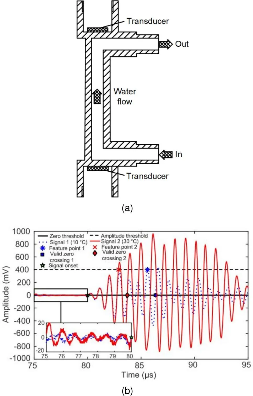
Fig. 1 Illustration on principle and problems of double-threshold method: (a) sensor; (b) experimental signal

The additional deviation certainly caused error in further computations. It should be recognized that for specified signals, there is always a proper threshold to ensure the feature points locating at the same cycle. However, it is difficult to find the proper threshold for signals under all conditions. Because many factors including fluid type and fluid temperature lead to variations in amplitude and waveform of ultrasonic signal which have been reported in many papers (Bravo et al., 1994; Zheng et al., 2016; Zhu et al., 2017; Fang et al., 2018), measurement conditions are unpredictable and it is not easy to find a proper threshold in some applications, such as those with wide temperature ranges.

It is notable that noise at a similar frequency to the signal was observed just before the onset of both signals, which will be further discussed.

3 Method

The proposed method can be recognized as complementary to the double-threshold method, and is aimed at eliminating the cycle-skip phenomenon. The approach is to estimate the onset point of the ultrasonic signal with the judgement factors for individual cycles of the signal, which are based on correlation coefficients and signal power. In this section, we will use signal 1 to introduce the method (Fig. 1) because of its typical defects including distorted waveform, the presence of noise at a similar frequency, and varied signal frequency.

3.1 Effectiveness and limitation of the correlation coefficient

In the proposed method, the received signal of an ultrasonic transducer is sampled and preprocessed. The signal is first debiased to facilitate further computations. Then, the double-threshold method is used to generate a feature point. The signal period where the feature point is located is selected as the reference period and labeled asref. The signal before the reference period is segmented into individual periods and labeled as1,2, …,, as shown in Fig. 2. Note that the number of periods should be large enough to ensure that the signal onset point is covered.

After preprocessing, correlation coefficients between each period and reference period are calculated. For two discrete sequences() and(), correlation coefficient(,) is defined as follows:

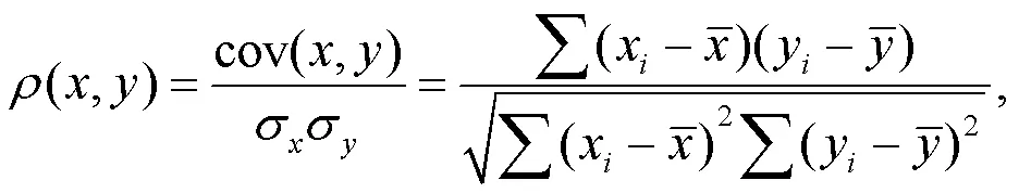
whereσandσare standard deviations of sequences() and() respectively. For periodp, the correlation coefficient is represented asρ, i.e.ρ=(p,ref),=1, 2, …,.

The correlation coefficient is a measurement of the coherence of two signals, indicating similarity between them. The more similar the sequences are, the closer to 1 (perfect positive correlation) or −1 (perfect negative correlation) the coefficient will be. For sequences with a weak relationship to each other, the coefficient will be around 0.

Since ultrasonic signal is a periodic sequence, the correlation coefficient between different periods of the signal is close to 1 and that between signal and noise is close to 0. This is effective for signal with high SNR or with different frequencies compared to the noise. For example, the correlation coefficients that result from replacing the noise in signal 1 with white Gaussian noise are shown in Fig. 3.

A sudden decline of the correlation coefficient can be observed in Fig. 3. On the basis of this phenomenon, the signal onset can be found and the TOF determined. This is the main principle of the method proposed by Wu et al. (2014). However, the decline becomes harder to distinguish when the noise and signal frequencies are similar. Fig. 4 shows correlation coefficients of signal 1 with original noise which has a similar frequency to the ultrasonic signal.

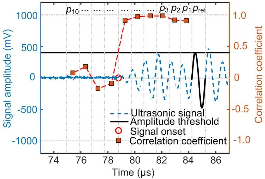
Fig. 3 Correlation coefficients of signal 1 with white Gaussian noise

3.2 Employment of signal power

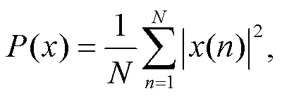
It is difficult to pick up the onset with only correlation coefficients, as shown in Fig. 4. Therefore, signal power is introduced into the method as the other parameter to derive the judgement factor. The average power of a discrete signal() is defined as follows:

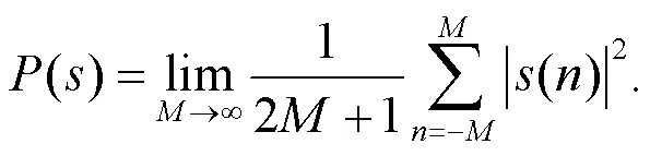
Since every single period of signal is defined in a finite length, the average power of periodic signals() is introduced, which equals the average power in one period. For a single cycle of ultrasonic signal(),=1, 2, …,, the average power is:

whererepresents the number of points in the corresponding period of signal. The power of each period of signal is calculated and labeled asP, i.e.P=(p),=1, 2, …,. Signal power is a measurement of signal strength. As noise usually has much lower amplitude than the periods of ultrasonic signal, there will be a great difference in signal energy before and after onset. The corresponding signal power for each period in signal 1 is shown in Fig. 5.

With the two parametersρandPcalculated, we can calculate the judgement factor byf=ρ·P. The corresponding judgement factors for signal 1 are shown in Fig. 6.

As a product of two parameters, the new judgement factor will show a significant decline as long as there is a decline in either parameter. In the case of noise with large amplitude but different frequency from the ultrasonic signal, there will be a sudden decline in the correlation coefficient, as shown in Fig. 3. In the case of noise frequency being similar to the ultrasonic signal but with smaller amplitude, the correlation coefficients might be close as shown in Fig. 4, but Fig. 5 indicates that there will be a sudden decline in signal power. Thus, the proposed method has a stronger anti-noise capability. A premise for the method is that signal must not have noise with both large amplitude and similar frequency near the onset, which is a reasonable condition for real applications. Otherwise, neither of the parameters will show a significant difference between ultrasonic signal and noise, and in fact, any method would fail to find the onset under such conditions.

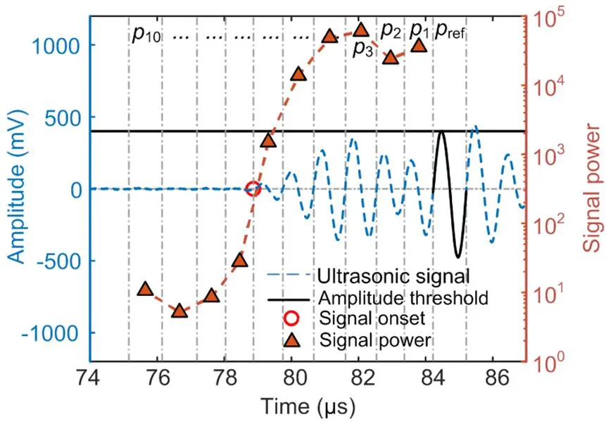
Fig. 5 Power of each period of signal 1

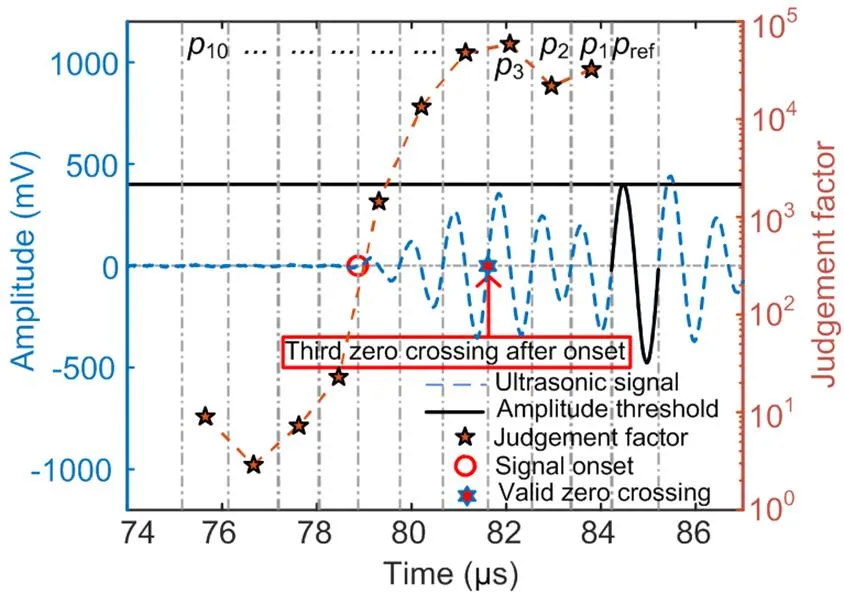
Fig. 6 Judgement factor of each period of signal 1

By detecting the sudden decline of the judgement factor, the first period of ultrasonic signal can be determined, i.e. the onset. Considering low SNR near the onset, the zero crossing that has a constant lag from the onset was selected to determine the TOF to guarantee the precision. As shown in Fig. 6, the third zero crossing after onset was selected as the valid zero crossing and the determined TOF was 81.75 μs.

3.3 Optimizations for varying signal frequency and low sampling rate

With regard to practical application, there are two problems with the proposed method. Details of the problems and corresponding solutions are described in this section.

3.3.1 Optimized segmentation method for varying signal frequency

Theoretically, the frequency of ultrasonic signal is stable from the onset to the end. This means that the number of points is always the same for every period in the signal with a fixed sampling rate. However, the actual frequency of ultrasonic signal usually varies. If a method which uses a fixed number of sampling points for segmentation is applied to an actual ultrasonic signal, the initial phase of each period will be different and this will cause an unexpected decline in correlation coefficients. Because an ultrasonic signal can be seen as a modulated sinusoidal wave, a sinusoidal function with time-varying frequency can be constructed to explain the problem.

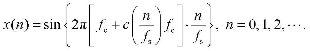
Assume that a sine wave is described as follows:

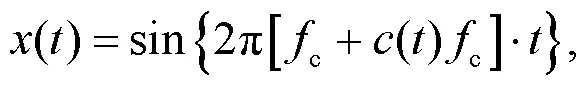
wherecis the nominal central frequency of the ultrasonic transducer and()crepresents frequency variation with time. Sample the signal at a frequencys=·c, and the obtained sequence can be described as:

If taking everypoints of data as one period, the initial phase of each period can be calculated by replacingin Eq. (5) with, where=0, 1, 2, …; then we can obtain the phase of theth period:

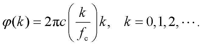
Eq. (6) shows that the phases of the periodsare varying along with their positions in the signal. Varying phase might cause an unexpected decrease in correlation coefficient, as shown in Fig. 7a. Consequently,1is mistaken as the first period of ultrasonic signal due to the unexpected decline.

To solve this problem, we optimized the method for signal segmentation based on zero-crossing detection. First, we detected the first zero crossing before the feature point as the start of the reference period, and labeled its index as0. For othersegmentations, additionalindices were needed. For signal with center frequencycand sampling rates=·c, indicesI,=1, 2, …,, could be determined by the following steps:

(i) Search zero crossing from the point (I−1−) to both sides within((I−1−),δ).δrepresents the maximum uncertainty of a signal period, which is determined by the transducer and sampling rate.

(ii) Take the index of the first zero crossing found asI, and take (I−1−) asIif no zero crossing is found.

After segmenting with the optimized method, a new problem appeared: that the numbers of points in different periods might be different. This prevented computation of a correlation coefficient, but the problem was solved by simply changing the length of the reference period to match the length of the period it was being correlated with. Results based on the optimized method are shown in Fig. 7b.

All discussions in the paper are based on experimental signals, and the optimization was adopted in the measurements above as well.

3.3.2 Employment of fast Fourier transform (FFT)-based interpolation for data with a low sampling rate

Regardless of the segmentation method, the sampling rate also has an influence on the initial phase of different periods. As it is almost impossible to sample every zero crossing, a segmented period always starts from a point near its positive zero crossing, so the uncertainty of the initial phase is:

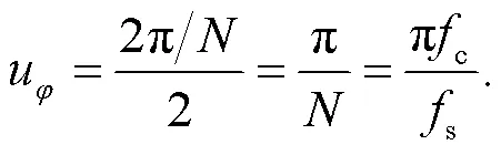
Eq. (7) shows that the uncertainty of initial phase for signal with specified frequency increases when the sampling rate decreases. This will also cause an unexpected decline in the correlation coefficient. Fig. 8 shows correlation coefficients for signal 1 with a sampling rate of only 5 MHz. Note that the original data was sampled at 100 MHz, and data with a low sampling rate was extrapolated from the original data by selecting one point every 20 points.

Correlation coefficients calculated with a sampling rate of 100 MHz show almost ideal characteristics (Figs. 3 and 4). While the data with a 5-MHz sampling rate shows an unexpected decline and causes error in the judgement in Fig. 8. However, it is impractical for an embedded system to reach such a high sampling rate. Actually, the sampling rate of an embedded system is rarely higher than 10 MHz. To solve the problem, FFT-based interpolation is employed here to improve the equivalent sampling rate.

Here we will give a brief introduction to FFT-based interpolation. The sampling rate of discrete signals in a time domain can be increased by inserting zeros in the frequency domain (Lyons, 2004). First, the ratio between the number of points of the sequence before interpolation and that after interpolation (the “interpolation factor”) is predetermined. In this method, the frequency-domain sequence of signal() is computed as(). According to the interpolation factor, a corresponding number of zero-valued sample points are inserted in the middle of() to generate a new sequence(). By conducting inverse fast Fourier transform (IFFT) on(), an interpolated time-domain sequence() is obtained.

After we improved the sampling rate of the signal from 5 MHz to 20 MHz by interpolation, the unexpected decline in correlation coefficients disappeared, as shown in Fig. 9.

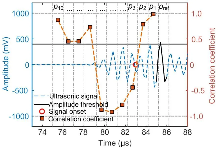
Fig. 8 Correlation coefficients of signal 1 with 5-MHz sampling rate

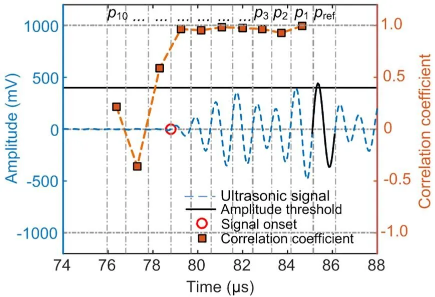
Fig. 9 Correlation coefficients of signal 1 with 20-MHz sampling rate interpolated from 5 MHz

3.4 Complexity analysis of the method

The proposed method is realized by four steps: interpolation, signal segmentation, judgement factor calculation, and TOF determination. The calculation burden mainly comes from interpolation and judgement factor calculation. Complexities of the two steps are calculated separately.

The interpolation consists of one-point FFT and one-point IFFT, whereandrepresent the number of points before and after interpolation. Thus, the complexity of interpolation is(·log()+·log()). Assume that there areperiods of signal to calculate judgement factors and each period containspoints. According to Eqs. (1) and (3), 6·of addition and 3·+of multiplication operations are needed in total. Thus, the complexity is(·).

As demonstrated in Figs. 3–9, 10 periods of signal and one period of reference are enough for calculation. As a result, we can obtain=55 for signal with a sampling rate of 5 MHz, as shown in Fig. 8, and=220 after interpolating to 20 MHz. Consequently,=10 and=20. With a definite number of points, the exact number of operations in our analysis can be determined as 8496 of addition and 5474 of multiplication. For digital signal processors (DSPs) such as TMS320C5535 with an instruction cycle of 10 ns, the time required for the proposed method is theoretically 0.1397 ms, which is still be far less than the typical output cycle of 10 ms of industrial ultrasonic flow sensors such as SFC-010T from TOKYO KEISO, Japan even after taking all other operations into consideration.

4 Experimental validation

Our proposed method is designed to suppress the cycle-skip phenomenon in ultrasonic flow measurement, which occurs frequently when the amplitude and waveform of received signal change. Thus, we applied the method under these conditions to verify its effectiveness.

As described in previous sections, many factors involving fluid type and fluid temperature have an influence on ultrasonic signal. Of these, fluid temperature has the most obvious effect on both amplitude and waveform of the signal (Bravo et al., 1994; Zheng et al., 2016). Thus, water temperature was chosen as the variable parameter in the experiment. On the other hand, the TOFs were expected to directly indicate whether cycle skip occurred or not. Thus, other settings of the experimental setup were kept unchanged and only downstream signals were sampled so that the TOFs would change smoothly with temperature if no cycle skip occurred.

Ultrasonic signal from a water flow sensor was sampled with a National Instruments (NI, USA) acquisition system, and the data was then processed with MATLAB on a PC. TOFs based on the double- threshold method and the proposed method were computed for validation.

4.1 Experimental setup

The experiment was carried out on a calibration system with an ultrasonic water flow sensor. A schematic of the experimental setup is shown in Fig. 10. The flow circuit consisted of a tank with a heater, a condenser, a pump, a manual valve, and a reference flow meter for flow adjustment. The flow sensor was connected in series in the circuit, and a temperature sensor was installed at the inlet of the flow sensor to record temperature during the experiment. The flow sensor was connected to an analog converter for signal conditioning, including filtering and amplifying. The conditioned signal was then sampled by an NI acquisition system, and the data was finally processed on a PC by MATLAB. The calibration system was custom made by the GANGYIN Flow Testing Equipment Company in Ningbo, China. The model and specifications of sensors used in the experimental setup are shown in Table 1.

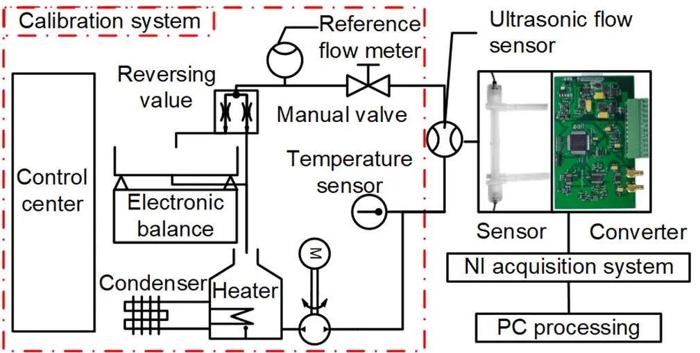
Fig. 10 Schematic of the experimental setup

The ultrasonic flow sensor used to sample signal was made by our team, and had a measurement tube made of perfluoroalkoxy alkane (PFA) and two ultrasonic transducers made of PZT-5H. Fig. 11 shows the structure of the sensor and Table 2 lists the values of corresponding parameters.

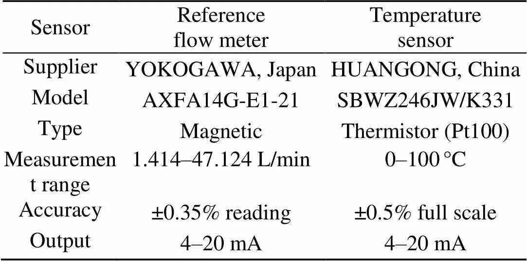
Table 1 Specifications of sensors used in the experimental setup

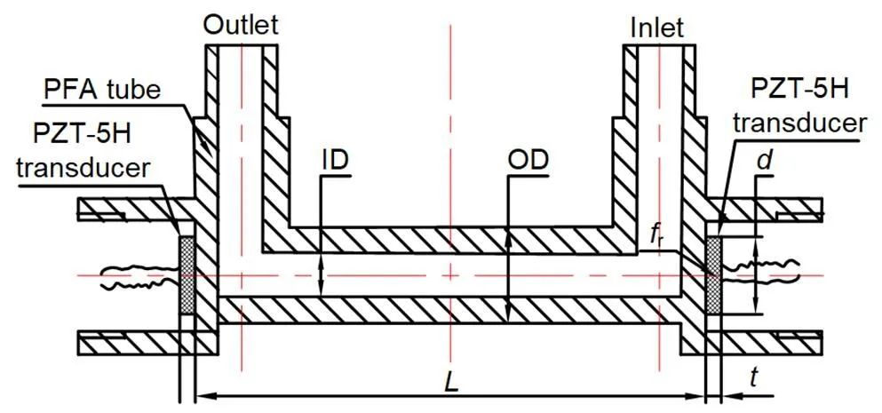
Fig. 11 Structure of the ultrasonic flow sensor

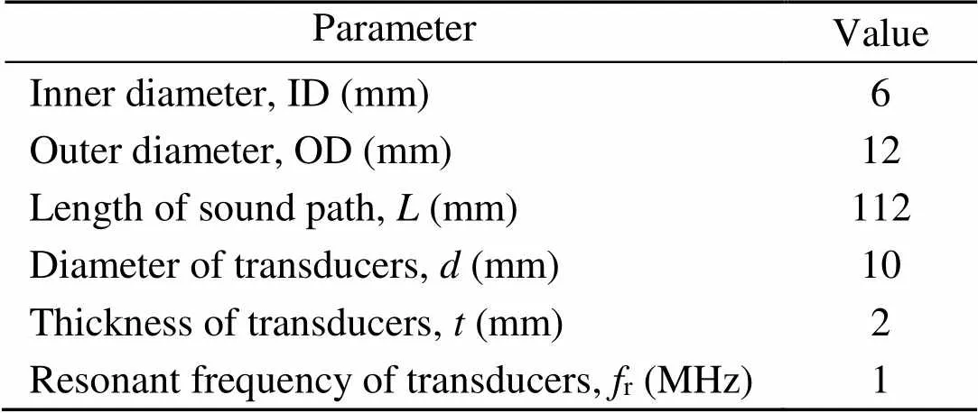
Table 2 Detailed parameters of the ultrasonic flow sensor

The transducers were excited by three sinusoidal pulses, with a frequency of 1 MHz and peak-to-peak amplitude of 20 V. Conditioned signal from the converter was sampled at 100 MHz. This high sampling frequency was set for pre-research. Data theoretically obtained at a low sampling rate could be easily produced according to the ratio between 100 MHz and the desired sampling rate (5 MHz was used for final computation). The water temperature was changed continuously from 10 °C to 70 °C by the condenser and heater. The manual valve was kept still and the pump was kept at the same rotation speed to maintain the flow rate at 4 L/min. Details of the experimental setup are listed in Table 3.

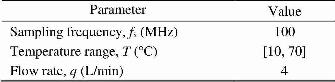
Table 3 Settings for the experiment

The flow circuit was first turned on and kept running at the set flow rate. At the beginning of the experiment, water in the tank was cooled down to around 8 °C by the condenser. Then, the heater started to work instead of the condenser to increase the temperature until the predetermined threshold was reached. The converter and acquisition system were turned on to record ultrasonic signal, and the water temperature was recorded accordingly. The acquisition system recorded one sequence of signal per second and only down-stream signal was recorded. The experiment ended when the water temperature rose over 70 °C and over 20 000 sets of signals were recorded.

4.2 Experimental results

With all signals sampled, we computed TOFs based on both the double-threshold method and the proposed method for verification. The amplitude threshold was set to a fixed ratio of the maximum signal value to prevent triggering failure.

Before computation, we reduced the sampling rate by selecting one point every 20 points, an equivalent sampling frequency to 5 MHz. This sampling rate can be easily implemented on an embedded system. Over 20 000 sets of data were acquired. As it is difficult to show all results clearly in one figure, 200 sets of data uniformly distributed from 10 °C to 70 °C were selected. The results are shown in Fig. 12.

As described above, only water temperature was varied during the experiment. Thus, we expected the TOF values to change smoothly with temperature if and only if the same zero crossing was used for all data. It is obvious from the dash curve in the figure that different zero crossings were used at different temperatures. The cycle-skip phenomenon occurred as temperature rose when the double-threshold method was used.

Fig. 13 shows signals at different water temperatures. Significant variations in both the amplitude and envelope of signal were observed. This explains why the cycle-skip phenomenon occurred when using the double-threshold method.

Note that the last cycle-skip phenomenon took place around 45 °C. In order to show the influence of the phenomenon on flow measurement, the ultrasonic flow sensor was calibrated at 43 °C and 49 °C. The instrument coefficient employed in the converter was first adjusted according to results of the double-threshold method at 43 °C and 4 L/min, and kept consistent in further calibrations. Calibration results are shown in Table 4.

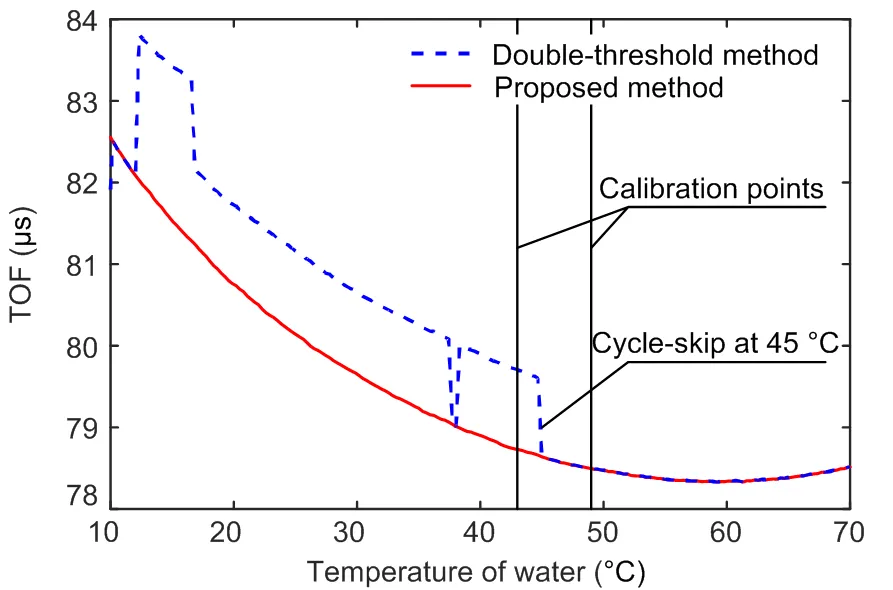
Fig. 12 TOF results based on double-threshold method and the proposed method

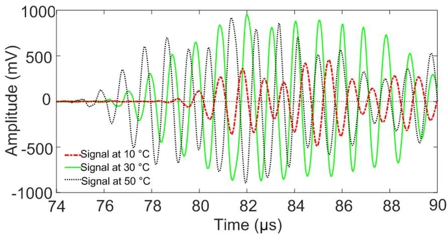
Fig. 13 Signals at different water temperatures

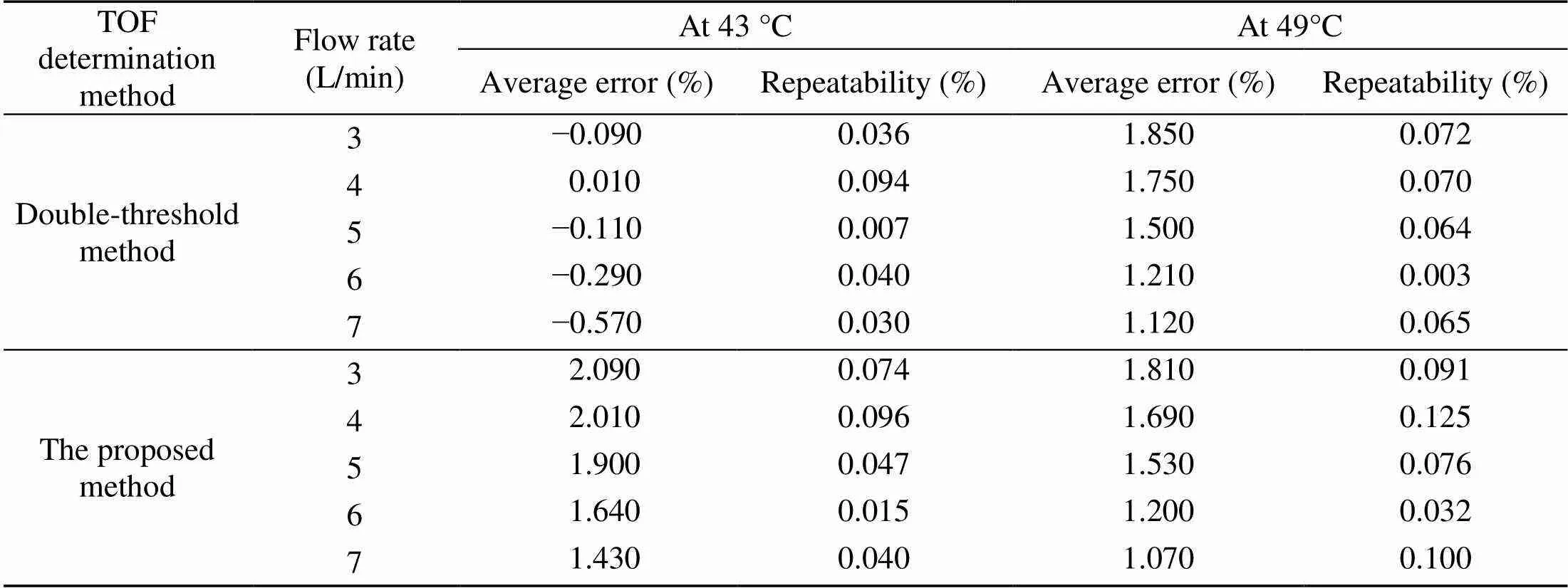
Table 4 Calibration results of the ultrasonic flow sensor at 43 °C and 49 °C

The average error of flow rate with TOF determined by the proposed method varied within 1% from 43 °C to 49 °C due to the variation of temperature. However, the variation in average error was nearly 2% when TOF was determined using the double-threshold method. Additional deviation was introduced because of the cycle-skip problem. A theoretical analysis of the errors in flow rate measurement follows.

In order to eliminate the influence of variation in sound speed caused by temperature, the flow rate can be calculated by

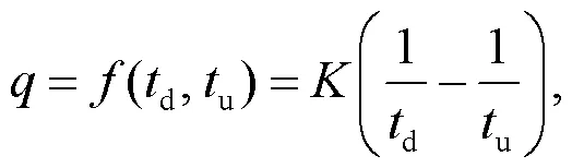
whereurepresents the upstream TOF,drepresents the downstream TOF, andrepresents the instrument coefficient of the ultrasonic flow sensor. Thus, the relative error ofcaused by variations inuanddcan be estimated by

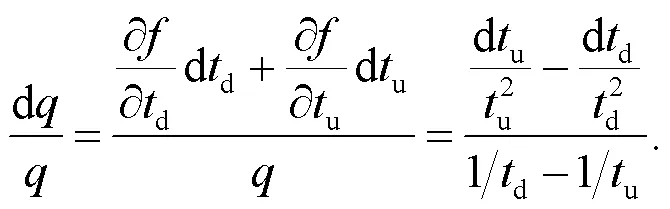
According to Fig. 12, where cycle skip occurred at 45 °C, we can obtain du=dd»−1 μs=dandu»d»79 μs. Then the relative error ofcan be calculated as

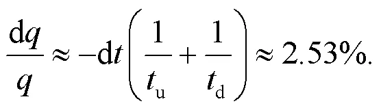
This is the error caused by one period of variation in TOF; the error would be greater if the cycle skip caused more periods of variation in TOF. To eliminate the additional error, the cycle-skip phenomenon must be avoided. The proposed method determines TOF by distinguishing ultrasonic signal periods and noise periods, so the result is independent of waveform variation. As shown by the solid curve in Fig. 12, the cycle-skip phenomenon was successfully suppressed by the proposed method.

5 Conclusions

The double-threshold method is still a commonly used method of TOF measurement because of its low cost and ease of implementation. However, performance of the method is negatively affected by the cycle-skip phenomenon. This paper proposes a method to suppress the phenomenon for reliable determination of TOF in ultrasonic flow sensors. First, the double-threshold method is employed to generate a feature point. Signal before the feature point is segmented into several individual periods. Next, judgement factors of these periods are calculated based on the correlation coefficient and signal power. The onset of ultrasonic signal is then determined by detecting the sudden decline of judgement factors. Finally, a valid zero crossing which has a constant lag from the onset is selected to determine TOF. The cycle-skip phenomenon is consequently suppressed. For better practicality, we also propose two modifications to solve the problems caused by varying frequency and low sampling rate of ultrasonic signal.

The proposed method has three main benefits: strong anti-noise capability due to the use of dual parameters, practicality due to the optimization skills, and robustness to signal waveform variation due to single-signal-based processing. A condition for successful use of the method is a lack of noise with both the same frequency and large amplitude near the onset point, which is reasonable for actual ultrasonic signals. We tested the method with an experiment based on an ultrasonic water flow sensor. Signals with increasing water temperature, i.e. with varying shape, were sampled and then processed using both the double- threshold method and the proposed method. The calculated TOF results prove that the proposed method is remarkably successful in suppressing the cycle-skip phenomenon.

Contributors

Ze-hua FANG raised the idea. Cheng-wei LIU completed and implemented the method. Yong-qiang LIU helped to build the experimental setup. Cheng-wei LIU, Liang HU, and Wei-ting LIU wrote the original draft. Rui SU and Liang HU revised and edited the final version.

Conflict of interest

Cheng-wei LIU, Ze-hua FANG, Liang HU, Yong-qiang LIU, Rui SU, and Wei-ting LIU declare that they have no conflict of interest.

Barshan B, 2000. Fast processing techniques for accurate ultrasonic range measurements., 11(1):45-50. https://doi.org/10.1088/0957-0233/11/1/307

Beck MS, 1981. Correlation in instruments: cross correlation flowmeters., 14(1):7-19. https://doi.org/10.1088/0022-3735/14/1/001

Bravo EC, Bastos TF, Martin JM, et al., 1994. Ultrasonics—temperature shapes the envelope., 14(4): 19-23. https://doi.org/10.1108/EUM0000000004234

Carullo A, Parvis M, 2001. An ultrasonic sensor for distance measurement in automotive applications., 1(2):143. https://doi.org/10.1109/JSEN.2001.936931

Demirli R, Saniie J, 2001. Model-based estimation of ultrasonic echoes. Part I: analysis and algorithms., 48(3):787-802. https://doi.org/10.1109/58.920713

Espinosa L, Bacca J, Prieto F, et al., 2018. Accuracy on the time-of-flight estimation for ultrasonic waves applied to non-destructive evaluation of standing trees: a comparative experimental study., 104(3):429-439. https://doi.org/10.3813/AAA.919186

Fang ZH, Hu L, Mao K, et al., 2018. Similarity judgment-based double-threshold method for time-of-flight determination in an ultrasonic gas flowmeter., 67(1):24-32. https://doi.org/10.1109/TIM.2017.2757158

Frederiksen TM, Howard WM, 1974. A single-chip monolithic sonar system., 9(6): 394-403. https://doi.org/10.1109/JSSC.1974.1050533

Hoseini MR, Wang XD, Zuo MJ, 2012. Estimating ultrasonic time of flight using envelope and quasi maximum likelihood method for damage detection and assessment., 45(8):2072-2080. https://doi.org/10.1016/j.measurement.2012.05.008

Hou HR, Zheng DD, Nie LX, 2015. Gas ultrasonic flow rate measurement through genetic-ant colony optimization based on the ultrasonic pulse received signal model., 26(4):045005. https://doi.org/10.1088/0957-0233/26/4/045005

Jiang YD, Wang BL, Huang ZY, et al., 2017. A model-based transit-time ultrasonic gas flowrate measurement method., 66(5):879-887. https://doi.org/10.1109/TIM.2016.2627247

Li WH, Chen Q, Wu JT, 2014. Double threshold ultrasonic distance measurement technique and its application., 85(4):044905. https://doi.org/10.1063/1.4871993

Lu ZK, Yang C, Qin DH, et al., 2016. Estimating ultrasonic time-of-flight through echo signal envelope and modified Gauss Newton method., 94:355-363. https://doi.org/10.1016/j.measurement.2016.08.013

Lynnworth LC, Liu Y, 2006. Ultrasonic flowmeters: half-century progress report, 1955-2005., 44(Sl): e1371-e1378. https://doi.org/10.1016/j.ultras.2006.05.046

Lyons RG, 2004. Understanding Digital Signal Processing,2nd Edition. Prentice Hall PTR, Upper Saddle River, USA, p.678-681.

Rajita G, Mandal N, 2016. Review on transit time ultrasonic flowmeter. The 2nd International Conference on Control,Instrumentation, Energy & Communication (CIEC), p.88- 92. https://doi.org/10.1109/CIEC.2016.7513740

Roosnek N, 2000. Novel digital signal processing techniques for ultrasonic gas flow measurements., 11(2):89-99. https://doi.org/10.1016/S0955-5986(00)00008-X

Sabatini AM, 1997. Correlation receivers using Laguerre filter banks for modelling narrowband ultrasonic echoes and estimating their time-of-flights., 44(6):1253-1263. https://doi.org/10.1109/58.656629

Sunol F, Ochoa DA, Garcia JE, 2019. High-precision time-of-flight determination algorithm for ultrasonic flow measurement., 68(8):2724-2732. https://doi.org/10.1109/TIM.2018.2869263

Tezuka K, Mori M, Suzuki T, et al., 2008. Ultrasonic pulse-Doppler flow meter application for hydraulic power plants., 19(3-4): 155-162. https://doi.org/10.1016/j.flowmeasinst.2007.06.004

Wu J, Zhu JG, Yang LH, et al., 2014. A highly accurate ultrasonic ranging method based on onset extraction and phase shift detection., 47:433-441. https://doi.org/10.1016/j.measurement.2013.09.025

Zheng DD, Hou HR, Zhang T, 2016. Research and realization of ultrasonic gas flow rate measurement based on ultrasonic exponential model., 67:112-119. https://doi.org/10.1016/j.ultras.2016.01.005

Zhu WJ, Xu KJ, Fang M, et al., 2017. Variable ratio threshold and zero-crossing detection based signal processing method for ultrasonic gas flow meter., 103: 343-352. https://doi.org/10.1016/j.measurement.2017.03.005

Journal of Zhejiang University-SCIENCE A (Applied Physics & Engineering)

ISSN 1673-565X (Print); ISSN 1862-1775 (Online)

www.jzus.zju.edu.cn; link.springer.com

E-mail: jzus_a@zju.edu.cn

© Zhejiang University Press 2021

https://doi.org/10.1631/jzus.A2000284

Revision accepted Mar. 3, 2021;

Crosschecked Sept. 6, 2021

TH71

June 24, 2020;

*Project supported by the Science Fund for Creative Research Groups of National Natural Science Foundation of China (No. 51821093)