Adjoint Method-Based Algorithm for Calculating the Relative Dispersion Ratio in a Hydrodynamic System

JI Fei, JIANG Wensheng, and GUO Xinyu,3)

1) State Key Laboratory of Satellite Ocean Environment Dynamics, Second Institute of Oceanography, Ministry of Natural Resources, Hangzhou 310012, China

2) Key Laboratory of Marine Environment and Ecology (Ministry of Education of China), Ocean University of China,Qingdao 266100, China

3) Center for Marine Environmental Studies, Ehime University, Matsuyama 790-8577, Japan

Abstract Relative dispersion ratio (RDR) can be used to quantify the deviation behavior of a water parcel’s trajectory caused by a disturbance in a hydrodynamic system. It can be calculated by using a standard method for determining relative dispersion (RD),which accounts for the growth of the deviation of a cluster of particles from a specific initial time. However, the standard method for computing RD is time consuming. It involves numerous computations on tracing many water parcels. In this study, a new method based on the adjoint method is proposed to acquire a series of RDR fields in one round of tracing. Through this method,the continuous variation in the RDR corresponding to a time series of the disturbance time t can be obtained. The consistency and efficiency of the new method are compared with those of the standard method by applying it to a double-gyre flow and an unsteady Arnold- Beltrami-Childress flow field. Results show that the two methods have good consistency in a finite time span. The new method has a notable speedup for evaluating the RDR at multiple t.

Key words relative dispersion; particle tracking; adjoint method; computational efficiency

1 Introduction

Particle tracking is widely used in oceanographic studies involving eitherin situobservation or numerical simulation. Its applications include rescue, marine oil spill detection, and marine environmental research (Hackettet al.,2009; García-Garridoet al., 2015; Kimet al., 2015). A good example of applying water parcel tracking is the autonomous Lagrangian current explorer float, which also plays an important role in ocean observations, such as the global ARGO program (Daviset al., 1992). Particle tracking is also used to find the source of certain substances distributed in seawater through backward tracking in various areas, including coasts and oceans (Durgadooet al.,2017; Gelderlooset al., 2017).

However, with particle tracking, a small disturbance on particles (either temporal or spatial) may cause a large path deviation. Particles released almost simultaneously at nearly the same location will exhibit dispersion behavior(Batchelor, 1952; Kuznetsovet al., 2002; LaCasce, 2008).Particles are normally assumed to be moving with the flow; as such, dispersion reflects the character of the flow field. Thus, the trajectory of a single particle is insufficient to represent the complete information about mass transport in seas. As a result, particle dispersion, which is caused by some mechanisms such as mixing in a hydrodynamic system, is also defined to characterize material transport and advection velocity (LaCasce and Ohlmann,2003; LaCasce, 2008).

To quantify the dispersion effect during particle tracking, Batchelor (1952) proposed the concept of relative dispersion (RD). LaCasce (2008) provided a simpler form that is described by releasing a cluster of particles in the vicinity ofx0at the initial timet0. The RD of pointt0at timeTwith disturbance att0is defined in Eq. (1) as the variance of the displacement of that cluster of particles

whereNis the total number of particles in a release experiment,t0is the releasing time,xi0(1 ≤i≤N) is the releasing position of theith particle at the initial releasing timet0in the vicinity ofx0. The operator || || is the norm in ann-dimensional Euclidean space and denotes the separation of particles from the center of mass (Batchelor,1952).x(T,xi0,t0) is the position of the particle at timeTreleased atxi0at the initial timet0. Ifxi0andt0are kept constant and onlyTvaries,x(T,xi0,t0) represents the trajectory of the particle being released at positionxi0at timet0.T,xi0andt0are commonly separated with either ‘|’ or‘;’ to reflect the Lagrangian characteristics and emphasize the varying feature of the variableTand the fixing feature of the particle positionxi0at timet0in defining the trajectory.T. In this studyT,xi0andt0vary together, so neither ‘|’ nor ‘;’ is used to avoid confusion.

RD is an important index used to describe the characteristics of particle separation. First, the value of RD represents the repelling (or attracting) feature of particles in a flow field. Second, the change in RD over the time elapsed after a disturbance may reflect different dispersion mechanisms (Kraichnan, 1966; Bennett, 1984). For example, if dispersion is dominated by eddies with the same scale as the particle’s separation distance, the growth of RD is in accordance with the power law. If dispersion is dominated by large-scale circulation, RD increases exponentially in time. If the separation between particles is larger than that in a circulation system, the motion of each particle shows an independent behavior that linearly increases RD with time. If the dispersion is caused by a random walk, RD is constant. Lastly, RD shows the sensitivity of a particle’s trajectory to its initial state,i.e., it is an index of the first kind of predictability (Lacorataet al., 2014).

D(T,x0,t0) depends on the initial distances among particles in a cluster. To eliminate the influence of the initial separation, we define the normalized RD as the relative dispersion ratio (RDR) as ,expressed asD(t,x0,t0)/D(t0,x0,t0), which is used to represent the dispersion feature of a flow field. The physical properties of RD (such as representing the repelling or attracting the features of particles and reflecting the mechanism of dispersion) can be inherited by the RDR. According to the form of the RDR,it is also an important intermediate variable,i.e., the square of the amplification factor of the distance between the particle pairs in the calculation of the finite time Lyapunov exponent (FTLE; Pierrehumbert and Yang, 1993).

The RDR or the derived variable FTLE has been applied to many oceanography problems. Sanderson (2014)verified the interface between a river and an ocean in an estuary in terms of the RDR calculated from a 3D flow field. Cuccoet al.(2016) used RDR to indicate the influence of wind data on the predictability of sea surface transport, which is crucial to maritime search and rescue operations. The spatial structure of the RDR is also utilized to explain water exchange in seas. For example,Fiorentinoet al. (2012) applied this method and explained the mechanism of sewage accumulation in coast water.Using high-frequency radar data and high-resolution sea surface drifter data, Shaddenet al.(2009) studied the exchange between water masses and calculated FTLE to verify the barrier effect of a high-FTLE ridge.

In observations and numerical experiments, the algorithm for calculating RD or RDR consists of two steps.First, a cluster of particles around one specific location is labeled at the initial time and each particle’s exact position is retained. Second, the RD in Eq. (1) is calculated by recording the displacement of the particles in the cluster as time proceeds. This ‘forward problem’ framework can capture a series of subsequent effects of a single initial disturbance, but it needs a considerable computation effort. To find the RDR at one point, at least two particles are tracked through integration. Normally, RDR spatial coverage is required to analyze the dispersion behavior of a flow field, and a considerable number of particles are needed to be deployed in the study area. Consequently, this process requires numerous computation tasks. Furthermore, many time instances or time spans, namelyt0andT,are required for the study, thereby enlarging the computation tasks.

In this study, a new method for calculating RDR is proposed by using the adjoint method to improve the computation efficiency of RDR. The adjoint method is a general approach to solve an inverse problem, which passes the derivative of one variable over state variables or some parameters backward to the whole process of a dynamic system (Le Dimet and Talagrand, 1986). In ocean studies,the adjoint method is widely utilized in sensitivity analysis, data assimilation, parameter estimation, optimal observation network design, and stability analysis (Errico,1997; Daescu and Langland, 2013).

In this study, the RDR derivedviathe new method is called Adj-RDR to be distinguished from the RDR based on the traditional method. In one round of calculation, a series of Adj-RDR fields can be obtained on the basis of particle dispersions at the final timeTbut with different initial timet. Thus, the potential disturbance at each time instancetto the final position of the particle at timeTis determined. The new method is applied to two ideal flow fields to verify its consistency and efficiency.

The remaining parts of the paper are organized as follows. The existing RDR acquisition methods based on the definition and flow mapping are introduced in Section 2.The derivation of the new algorithm based on the adjoint method is also described in Section 2. Two ideal flow field experiments for the verification of our new method are demonstrated in Section 3. The results are discussed in Section 4, and the conclusions are presented in Section 5.

2 Methods

In Section 2.1, the standard RDR calculation method is presented to explain the new method. An algorithm based on flow mapping (Haller, 2002) is also proposed to extend the RDR as a continuous spatial function of the initial state. In Section 2.2, the new algorithm based on the adjoint method for calculating RDR is introduced.

2.1 RDR Calculation Based on a Standard Algorithm

The trajectory of a particle in a flow field is controlled by the following equation:

whereu(x(t～,x～,t),t～) denotes the velocity of the particle

In Eq. (1), RD is calculated on the basis of the relative displacement amongNparticles. It involves the distance betweenN(N-1)/2 pairs of particles. To simplify the derivation without losing generality, we define the distance of an arbitrary pair of particles as

d(T,xt,t) changes with the norm of disturbance ||Δxt||and the direction of disturbance Δxt/||Δxt||. Therefore,R(T,x0,t0) is a statistical variable, although it is normalized with the arithmetic average ofdi,j(t,x0,t0) = ||Δxt||2.

Haller (2002) provided a definition with a higher certainty by using the Cauchy-Green strain tensor atxt

where the eigenvalueλiindicates the extension rate of the distance between the particles in a pair in the direction denoted by the eigenvectorξi.

Dispersion is led by the maximum eigenvalue in the direction of the corresponding eigenvector; as such, the maximum eigenvalue is often used as the index of the square of the amplification factor of the distance between the particles in a pair in the calculation of FTLE (Haller,2002). In our study, the same notion is applied to calculate RDR:

The calculatedR(T,xt,t) corresponds to the maximum RDR among all the initial displacement directions. In this study, the method described in this section is called the standard method.

2.2 RDR Calculation Based on the Adjoint Method

First, a set of cost functionsJk,k= 1, 2,···,nis defined as follows:

Accordingly, a set of functionals with the constraints can be defined as

Eq. (14) is integrated by parts to obtain

When the Jacobi operator is applied to Eq. (17), and Eq. (16) is inserted, the following equation is derived:

where

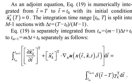
The left-hand side is discretized with an implicit timeforward scheme. The right-hand side can be integrated analytically by considering a Dirac function in the integrand.Thus, the numerical scheme of Eq. (19) is expressed as follows:

The RDR expressed in Eq. (11) can be obtained based on the Jacobian of flow mapping in Eq. (26). In this way,the influence of the disturbance at a series of time instancetmto the final location of the particle can be determined efficiently by evaluating the gradient of the flow field along the trajectory.

The calculation of RDRviathe adjoint method can be divided into four steps:

1) Place a numerical particle on every grid point in the study area at a certain initial time.

2) Track each particle in the flow field from the initial time to the final timeT,and keep the position of the particle at timetm,xtiand ∇xu(i)at the same point at the same time, wherei= 1, 2,···,M.

3 Application of the Proposed Method in Two Ideal Flow Fields

In particle tracking studies, two common questions are commonly encountered. One is, ‘what is the final particle distribution that can occur due to the disturbance at time(named as disturbance timet0)?’. The other one is, ‘what kind of disturbance att0can cause the final distribution of particles?’. The first one is called the forward tracking problem, which can be used to describe the spreading of pollutants at a certain time (named as result timeT) and being discharged at differentt0,e.g., different phases of a tidal period. The second one is called the backward tracking problem, which can be utilized in instances such as locating the oil spill source att0from the oil coverage in water atT. In both cases the final timeTis normally regarded as a fixed value, andt0is assumed as a varying variable. The RDR field at a continuously varyingt0is required to solve these problems.

The RDR in the two problems can be obtained by using the traditional method described in Section 2.1. They can also be more efficiently solved by applying the new method presented in Section 2.2. In this section, two widely used analytical flow fields, namely, two- dimensional double-gyre flow and three-dimensional unsteady ABC flow,are adopted to verify the validity and efficiency of the new method proposed in Section 2.2. These flow fields are benchmark models for studying the Lagrangian chaos and mixing either 2D (Shaddenet al., 2005; Coullietteet al., 2007) or 3D dynamic systems (Dombreet al., 1986;Haller, 2001). In the present study, two- dimensional double-gyre flow and three-dimensional unsteady ABC flow are used in forward and backward tracking problems, respectively. The RDRs of these two flow fields at different initial times are calculated by using the standard method and the newly proposed adjoint method. The results of both methods are compared to verify the effectiveness of the new method.

For the convenience of reference, the RDRs calculatedviathe new method and the standard algorithm are called Adj-RDR and standard RDR, respectively.

3.1 Double-Gyre Flow Case

In this section, the forward tracking problem is solved for a double-gyre flow field. This flow field is designed as two adjacent closed gyres flowing at a constant speed.They are separated by a straight line named as the flow axis, which oscillates periodically with a small amplitude so that the two gyres can expand and contract alternately.

The flow field is given by

Fig.1 RDR of the double-gyre flow calculated by two methods. Column A, RDR calculated by the standard algorithm displayed as log10RDR; Column B, RDR calculated by the adjoint method, displayed as log10RDR; Column C, The absolute difference between RBR calculated by two methods. Rows 1 to 6 denote the results with initial disturbance time at 0, 4, 8, 12, 16 and 20.

Adj-RDR is calculated in accordance with the procedure described in Section 2.2 at a time step of 0.02. The reason for taking this value of Δtis explained in the discussion. Six figures att0= 0, 4, 8, 12, 16, 20 are selected and presented in column B of Fig.1, which shows the RDR distribution with the same meaning as those in column A. However, the RDRs of differentt0are calculated by tracking the particles in one run. In Fig.1, the spatial pattern of Adj-RDR is consistent with the result of the standard algorithm. Their difference is less than 15% of the absolute value in column C of Fig.1, but Adj-RDR is higher than the result obtainedviathe standard algorithm.The overestimation of Adj-RDR occurs in the low- value region of RDR,e.g., the center of the gyres. The difference between the two algorithms in a high-value area,where we are usually most interested in, is smaller than that in a low-value area. Therefore, the result of Adj- RDR is acceptable in the double-gyre test.

The area-averaged RDRs obtained with both methods are also compared in Fig.2. Adj-RDR is calculated at a time step interval of 0.02, so it is represented as a continuous line. The RDR based on the standard algorithm is shown as 6 points in the figure. Whent0＞ 8,i.e., the track span is shorter than 12, Fig.2 shows a good correspondence between the two RDRs based on different algorithms. The value producedviathe new methodis higher than that obtainedviathe standard method. Ift0＜ 8,i.e.,the track span is longer than 12, then Adj-RDR exponentially grows with the track span, but the standard RDR appears to reach the maximum value at 107.

The computation time consumed by using the two methods is compared. A desktop computer with a 3.6 GHz AMD 3700x processor is used to calculate the RDR with MATLAB 2017b. ‘Tic’ and ‘toc’ commands are utilized to keep time. The computation time is the average of the results of three rounds of calculations. The standard method takes 138.1 ± 0.5 s to obtain the distribution of the RDR in six cases (t0= 0, 4, 8, 12, 16, 20). By comparison, the adjoint method needs 136.0 ± 0.5 s to determine the distribution of the RDR in 100 cases att0of 0 to 20 with a time step of 0.2.

Fig.2 Area averaged RDRs calculated by both methods continuous line, Adj-RDR; point, RDR by standard algorism.

3.2 Backward Tracking in an Unsteady ABC Flow

As mentioned at the beginning of this section, the RDR can be used to determine the source of matter in oceans by solving the backward tracking problem. In the application of backward tracking, a new flow field is formulated by reversing the time sequence and taking the opposite sign of the original flow field. Thus, a new flow mapping is defined as

Then, the RDR can be calculated for this flow mapping by using the standard algorithm or the adjoint method as the forward tracking problem.

The physical definition of the derived RDR differs from that obtained through forward tracking, as in Section 3.1.The high RDR, in this case, indicates the area where particles gather (Haller, 2015).

In this section, the unsteady ABC flow is used as the test flow field, which is given by

The original backward tracking problem here is to find the disturbance attthat can generate the end state atT. In the transformed forward problem, the goal is to obtain the RDR whent～ is from 0 to 8 and the final state isT～ =8.When the standard algorithm is usedt～= 0, 0.4, 0.8, 1.2,1.6, that corresponds tot～= 8, 7.6, 7.2, 6.8, 6.4 is chosen.When the new adjoint method is applied,t～ is selected from 0 to 8 with a time step of 0.02.

The RDR distribution on the three surfaces of the calculation cube is shown in Fig.3 whent～ =0,i.e.,t=8 is chosen. The results from the standard algorithm and the adjoint method are presented in Figs.3a and 3b, respectively. They display the ‘hollow’ pattern of a high value around the vortex tube. However, the RDR obtained with the adjoint method has a ‘higher contrast’ than that determined with the standard algorithm. Therefore, Adj-RDR is higher than the standard RDR in the high-value zone,whereas the former is lower than the latter in the lowvalue zone. This pattern can also be found in Fig.3c, which shows the difference between the RDRs acquired by both methods.

The RDR distribution at different initial times on the three slices in the middle of the cube,i.e.,x1= π,x2= π,andx3= π, is plotted to express the results more clearly.The RDRs calculated by the standard algorithm and the adjoint method are displayed in Figs.4 and 5, respectively.Both RDR distributions are similar. However, the RDR in

Fig.5 has a ‘higher contrast’ than that in Fig.4. Furthermore, the RDR distribution in Fig.5 becomes blurrier as the time span betweent0andTis prolonged.

The time series of area-averaged Adj-RDR and standard RDR are shown in Fig.6. Adj-RDR exponentially grows astincreases. By comparison, the standard RDR grows exponentially whent＜ 6; as it reaches the maximum value, it no longer grows astincreases.

The time consumed by using the two methods in the ABC flow is compared. It is a 3D flow field, so the computation time is very long. For this reason, a parallel MATLAB m file is written and run in 10 threads. With the standard method, obtaining the RDR field in 1 case witht= 8 takes 1331.3 s. With the adjoint method, determining the distribution of the RDR field in 400 cases withtfrom 8 to 0 needs 2354.7 s.

Fig.3 RDR distribution of unsteady ABC flow field on three surfaces of the cube. (a), RDR calculated by the standard algorithm as log10RDR; (b), RDR calculated by the adjoint method as log10RDR; (c), the absolute difference between RBR calculated by two methods time range is for T = 0 and t0 = 8.

Fig.4 RDR distribution of unsteady ABC flow field calculated by the standard algorism on three inner sections of the cube with different initial time. The first row denotes x1 = π; second row denotes x2 = π; third row denotes x3 = π. The columns from 1-5 correspond to the initial time t = 8, 7.6, 7.2, 6.8 and 6.4. The color in the figures denotes the value log10RDR.

Fig.5 Same as Fig.4, but calculated by adjoint method.

Fig.6 The time series of area-averaged Adj-RDR and standard RDR. The red line denotes the continuous time series of the sum of Adj-RDR change with different initial time and the black dots denotes the sum of RDR calculated by standard algorithm. Each dot is averaged from an independent experiment with the disturbed particles released at t.

4 Discussion

4.1 Computational Efficiency

The RDR field calculated with the adjoint method is almost continuous with respect to. By contrast, the RDR field obtained with the standard method is confined to a certain instance oft. The calculation procedure needs to be carried out several times to determine the influence of disturbance from timettoT. Therefore, the new method is beneficial. The computational complexity of the two methods is briefly analyzed in this section.

In the standard method, particle tracking is the most time-consuming procedure. In the adjoint method, particle tracking and the calculation of Eq. (26) are both time consuming. Either particle tracking or particle tracking plus Eq. (26) consumes more than 90% of the calculation time of the corresponding method in the two examples in Section 3. Therefore, we focus on the comparison of the computational complexity of particle tracking and the calculation of Eq. (26).

The calculation cost of tracking one particle in annd-dimensional space in one time step needs at leastO(nd2)multiplications when a simple discrete form of Eq. (2),i.e.,Eq. (28), is used to track the particle:

Every calculation of Eq. (28) is assumed as one unit of calculation here. By using the standard method,nd+ 1 particles should be tracked in thend-dimensional space to determine the RDR by calculating Eq. (6) at one point. Ifnttime steps are needed to track a particle fromt0toT,then the computation cost to obtainR(T,x0,t0) isnt× (nd+1). The computation cost isnt× (nd+1) ×nrfor the disturbance at a single time instancet0to determine the RDR field withnrsampling points. If a series of RDR fields is needed with respect toncdisturbance time instances,e.g.,the 6 cases in Section 3.1,ncindependent calculations with different tracking time steps are needed. The disturbance time necessary.tis spread evenly betweent0toTfornccases. Then, the time step number in each case decreases fromntto 0, whiletis fromt0toT. Therefore, the total computation time to complete the whole calculation isnc/2 ×nt× (nd+ 1) ×nr.

In the adjoint method, the computation cost includes the computation of Eq. (26) and the computation of particle tracking. The computation cost of Eq. (26) isndtimes of Eq. (28). Particle tracking should be calculated fromt0toT(ntsteps) and the calculation of Eq. (28) fromTtot0(ntsteps) to acquire the RDR by using the adjoint method at one point. Therefore, for the continuous time series of Adj-RDR field atnrpoints, the computation cost isnt×(nd+1) ×nr.

Theoretically, the adjoint method saves the computation costnc/2 times of that of the standard method in solving the inverse problem. In real calculation, the adjoint method needs to record and read the data of particle position and velocity, so the calculation time tends to be longer than the theoretical value. The speedup is less thannc/2,but it is still very notable. In this study, the speedup ratio of the double-gyre example is about 16.9 times, which is less than 50 times in theory. For the unsteady ABC flow,the speedup ratio is about 113 times, which is also less than 200 times in theory.

In addition to time cost, the memory cost of the adjoint method is determined to calculate the RDR. The extra random-access memory (RAM) occupied by the Adj- RDR method mainly occurs in step 3 of the calculation procedure. In step 3, memory needs to save the spatial divergence tensor of the velocity for each particle of the current time step. The tensor isdtimes larger than the velocity vector, wheredis the spatial dimension; as such, the RAM usage of step 3 is alsodtimes of the particle tracking process. For the double-gyre experiment in Section 3.1, the tensor takes up 15.305 megabytes of RAM.

Apart from the RAM usage, extra disk space is required in the Adj-RDR method to record the trajectory information compared with that in the standard method. The data size of the trajectory can be expressed as follows:

File’s data size = Number of time steps × Number of released particles × Dimension of flow filed (float data).

The adjoint method requires a relatively high resolution in space and time, so the footprint of the trajectory information is a large amount of data. In the case of the double-gyre experiment in Section 3.1, the total size of the trajectory files is 6.872 gigabytes. In general, the extra cost of RAM and disk space is acceptable.

4.2 Computation Accuracy

Adj-RDR has the same spatial structure as that calculated by the standard algorithm in forward and backward tracking applications, as displayed in Section 3. However,Adj-RDR is higher than the standard RDR, especially when the calculation span is large. In the time series of the area-averaged Adj-RDR and standard RDR shown in Figs.2 and 6, Adj-RDR exponentially grows as the calculation time span increases. For the standard RDR, the dispersion ratio grows exponentially during a limited time;afterward, the area-averaged RDR appears to reach the maximum value. This difference occurs because the adjoint method calculates the tangent linear dispersion ratio in the smallest neighborhood along the particle trajectory.In the standard algorithm, the initial pair is finally separated into two tracks regardless of the size of the initial disturbance because of the effect of the dispersion. When the particle pairs are apart far enough, the relative motion between the particle pairs is basically random. Statistically, the average distance is no longer growing. Ding and Li (2007) explained the saturation phenomena in the study on the nonlinear FTLE. If the initial disturbance is small,the standard RDR is consistent with Adj-RDR in a longer time (Fig.7).

The RDR obtained by the adjoint method is sensitive to the time step in the calculation because of the tangent linear approximation. A set of experiments of the double- gyre flow field (as in Section 3.1) is used to discuss the relationship between the time step Δtand the Adj- RDR. A standard algorithm with the initial disturbanceδx= 10-5is used as a benchmark result. Figs.8 and 9 illustrate the influence of different time steps on the difference in the two methods. The smaller the time step, the smaller the difference in the RDR between the two methods. Moreover,in Fig.9, the difference increases when Δt= 0.032. Thus,when Δtis larger than the upper limit, the difference increases rapidly with Δt. However, when Δtis less than the time step, the decrease in Δtslightly affects the reduction in the difference. In the above experiment, Δt= 0.02 is used for the compromise between efficiency and accuracy.

Fig.7 Same as Fig.2, but the results of the standard RDR with a smaller initial disturbance scale are supplemented.The red line represents the RDR at each initial time calculated by the adjoint algorithm. The blue, cyan, and yellow dots correspond to the RDR calculated by the standard algorithm, and the initial distances between the particle pairs are 10-5, 10-6, and 10-7, respectively.

Fig.8 Absolute difference between Adj-RDR and standard RDR (Fig.1A). Columns A, B, C, D, and E denote the results obtained via the adjoint method with time steps of 0.002, 0.008, 0.032, 0.128, and 0.512, respectively. Rows 1 to 6 denote the results with initial disturbance times at 0, 4, 8, 12, 16, and 20.

Fig.9 Sum of the absolute difference between Adj-RDR and standard RDR, and the change with time step.

4.3 Limitations of the New Method

The RDR calculated by the adjoint method is blurrier in distribution as the time span betweent0andTis prolonged (Fig.5). Therefore, the accuracy of the new method is limited when the time span is long.

The reason for the time span limitation is thatR(T,xt,t)is calculated on the particle in the adjoint method,i.e.,RDR is mapped onxt, which varies witht. For comparison, in the standard method, RDR is mapped on the initial location where the particle is released. In an aperiodic flow field, whentis farther away fromt0,xtis farther away from the mesh point where the particles are released(Fig.10). In the area near the boundary, some particles leave the study area. In other words, the number of sampling points in the study area is reduced, and the distribution of sampling points is not uniform whent-t0is high.This effect is more significant for the flow field with an open boundary because particles eventually flow out of the study area.

However, if a study aims to calculate the structure of the RDR in a finite time, such as several tidal periods, the adjoint method is valid for the application.

5 Conclusions

In this study, a new method for calculating RDR is proposed by using the adjoint method. The validity of the method is verifiedviatwo idealized numerical experiments. The results reveal that the spatial structure of RDR calculated with the adjoint method is consistent with that obtained with the standard algorithm. The new method is successful in forward and backward tracking cases. Its computational efficiency is also exhibited with a speedup of more than 15 times in the two examples.

Fig.10 Adj-RDR distribution of the unsteady ABC flow field mapped on the location of a particle.

The new method has some limitations. The spatial resolution of RDR decreases as the tracking time is extended.Moreover, RDR increases as the integration time is prolonged. In many cases, this limitation can be avoided because the RDR of a finite time is needed. RDR calculated for a long time loses its physical significance because of the nature of the flow field itself.

In conclusion, the newly developed method for computing RDRviathe adjoint method can provide the time evolution of the dispersion characteristics of a flow field.The present study helps elucidate the mass or momentum distribution in seas. In future studies, the new method will be applied to real cases in oceans.

Acknowledgements

Fei Ji thanks the China Scholarship Council (CSC) for supporting his stay in Japan and the Ministry of Education,Culture, Sports, Science and Technology, Japan (MEXT)under a Joint Usage/Research Center, Leading Academia in Marine and Environment Pollution Research (LaMer)Project for supporting his short stay in Japan.